-
-
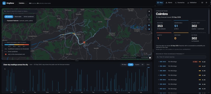
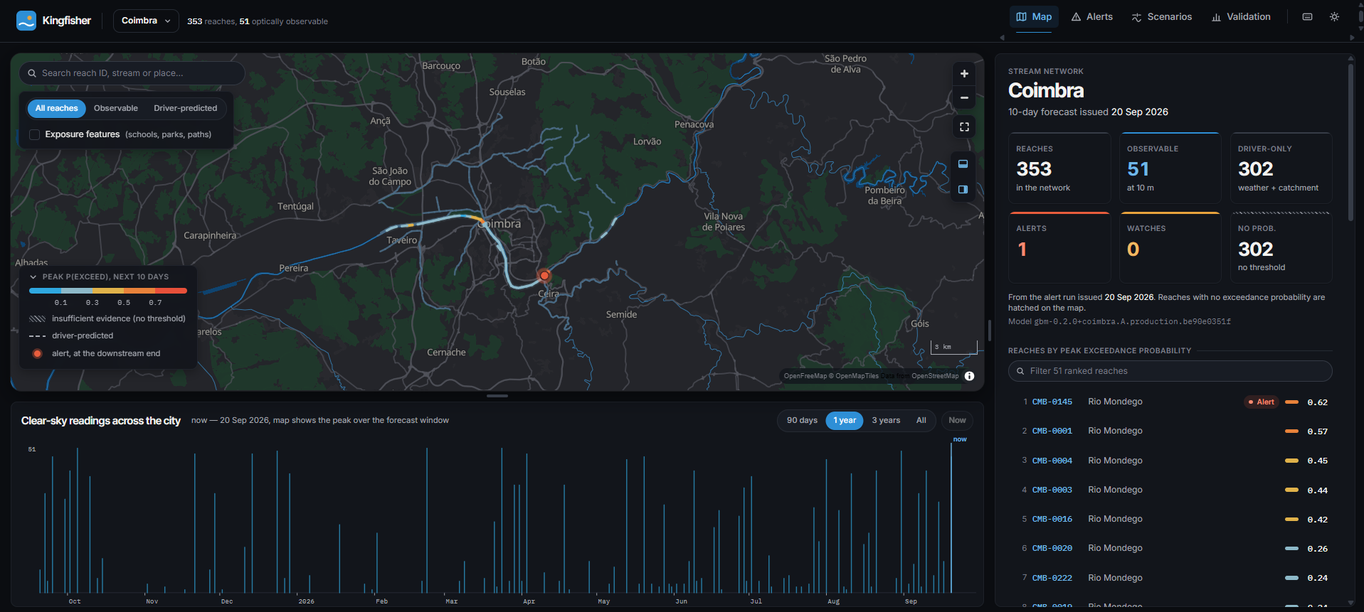
Kingfisher: early warning and resilience planning for urban streams. (dark theme)
-
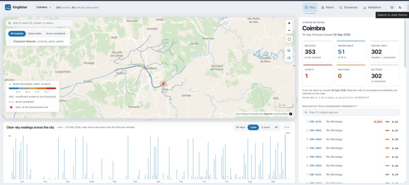
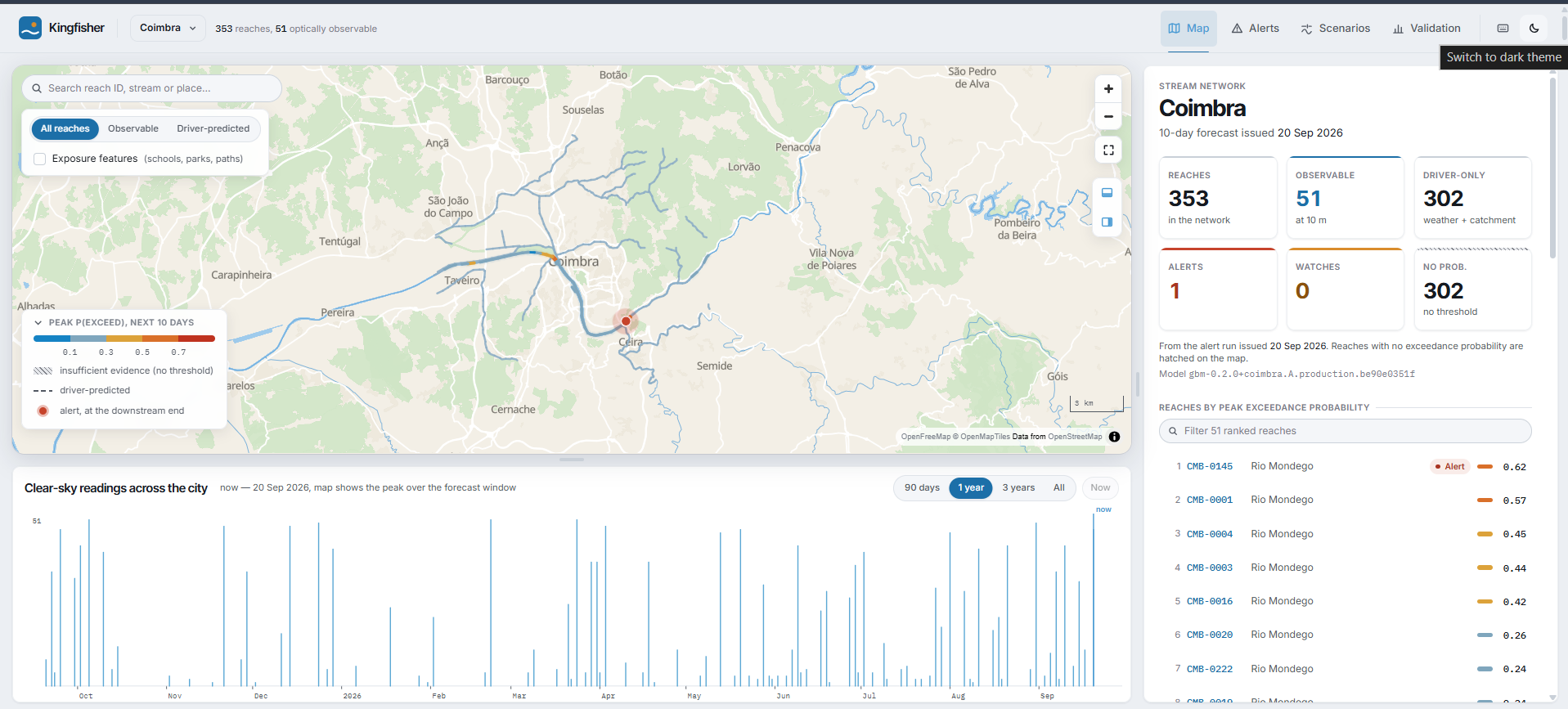
Coimbra overview: 353 reaches, 51 visible to Sentinel-2 at 10 m. 302 are forecast from weather and catchment data but capped at Watch.
-
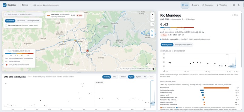
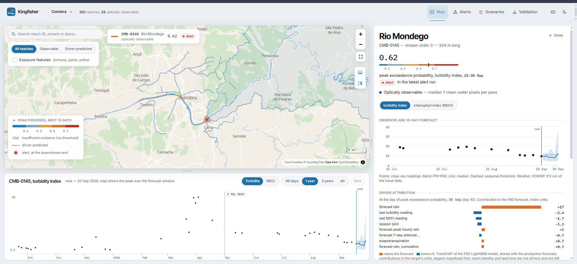
Reach detail: past clear-sky readings, a 10-day P10–P90 forecast against the seasonal threshold, and the drivers behind the peak.
-
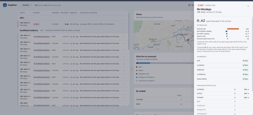
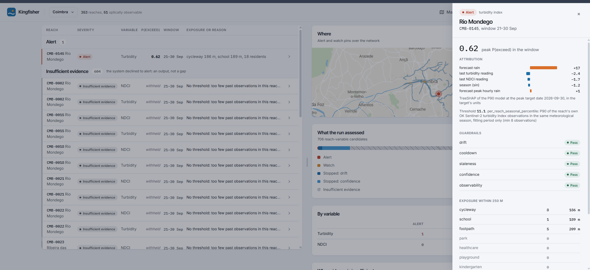
Alert CMB-0145: P(exceed) 0.62 with TreeSHAP drivers, all 5 guardrails passed, and the schools and paths within 250 m.
-
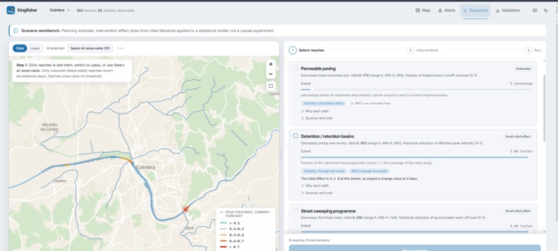
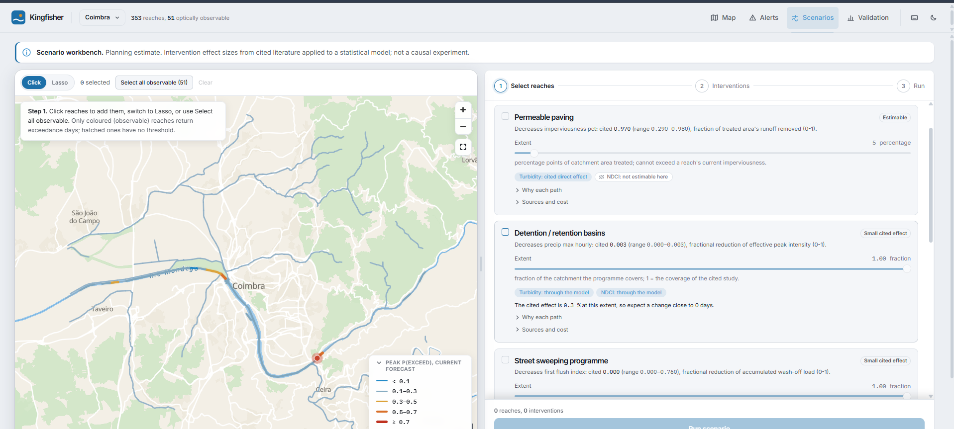
Scenario workbench: pick reaches, then apply cited levers. Each lever is labelled estimable, small cited effect or not estimable here.
-
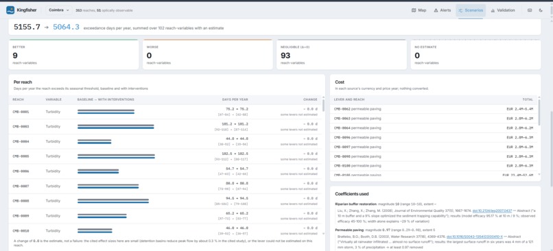
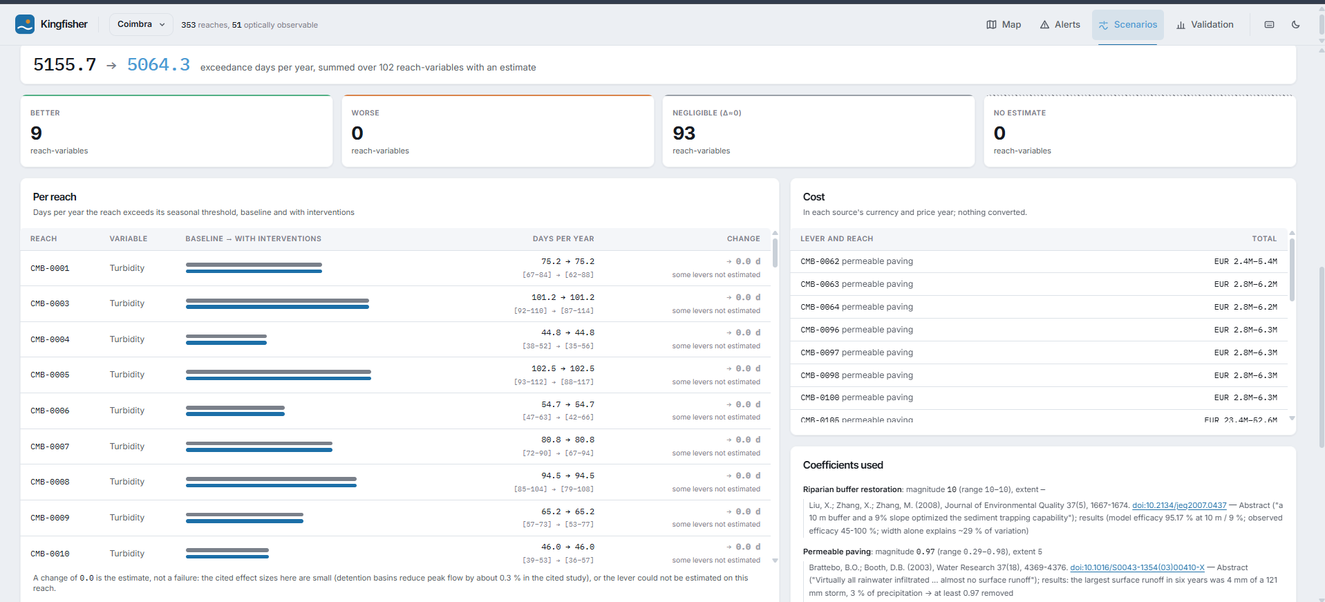
Scenario result: exceedance days per reach with intervals. 9 reaches improve, 93 show Δ≈0. Costs stay in each source's own currency.
-
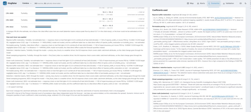
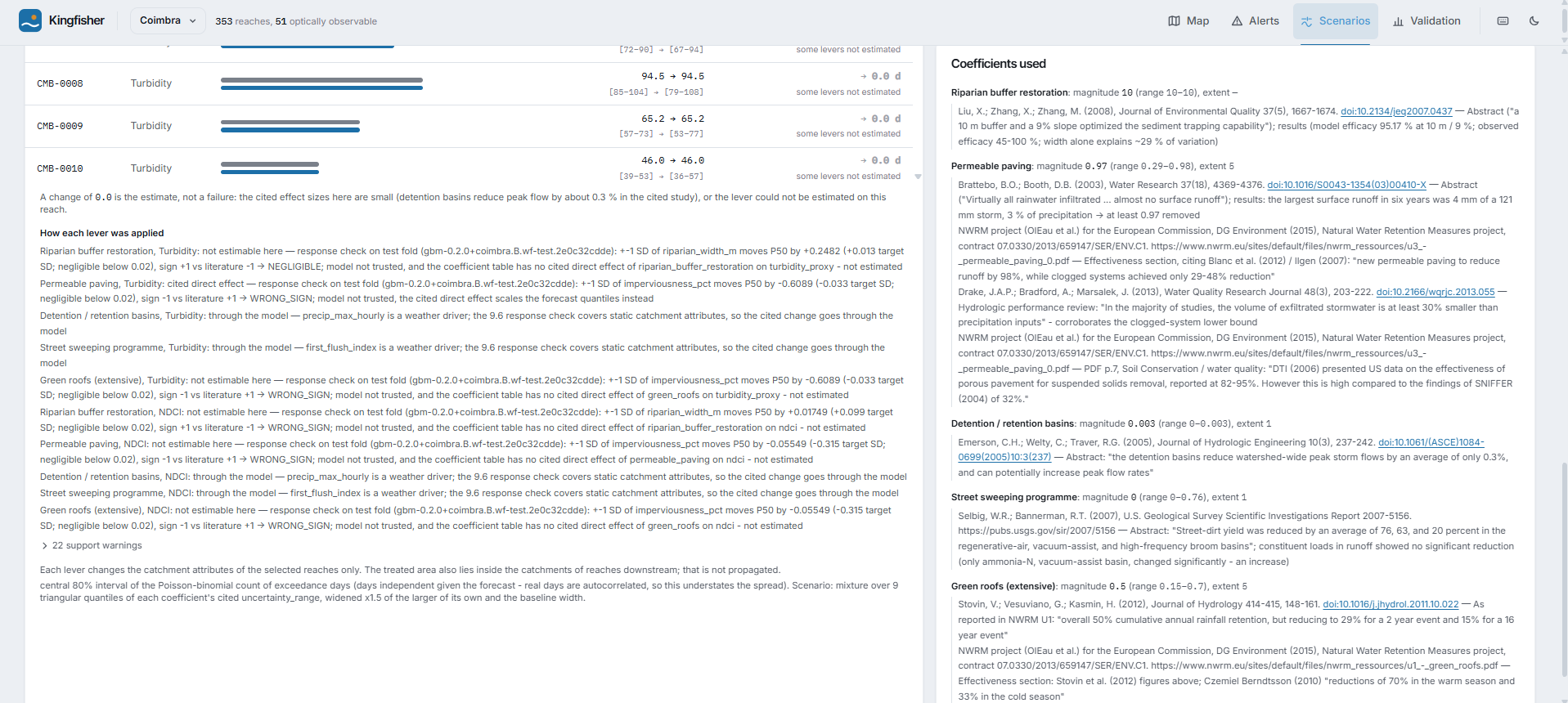
Scenario audit: every lever shows its path (model, cited direct effect or not estimable) and its citation, DOI and quoted evidence.
-
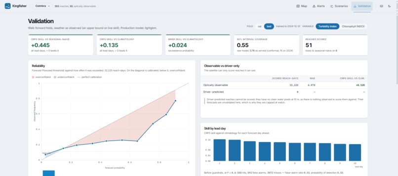
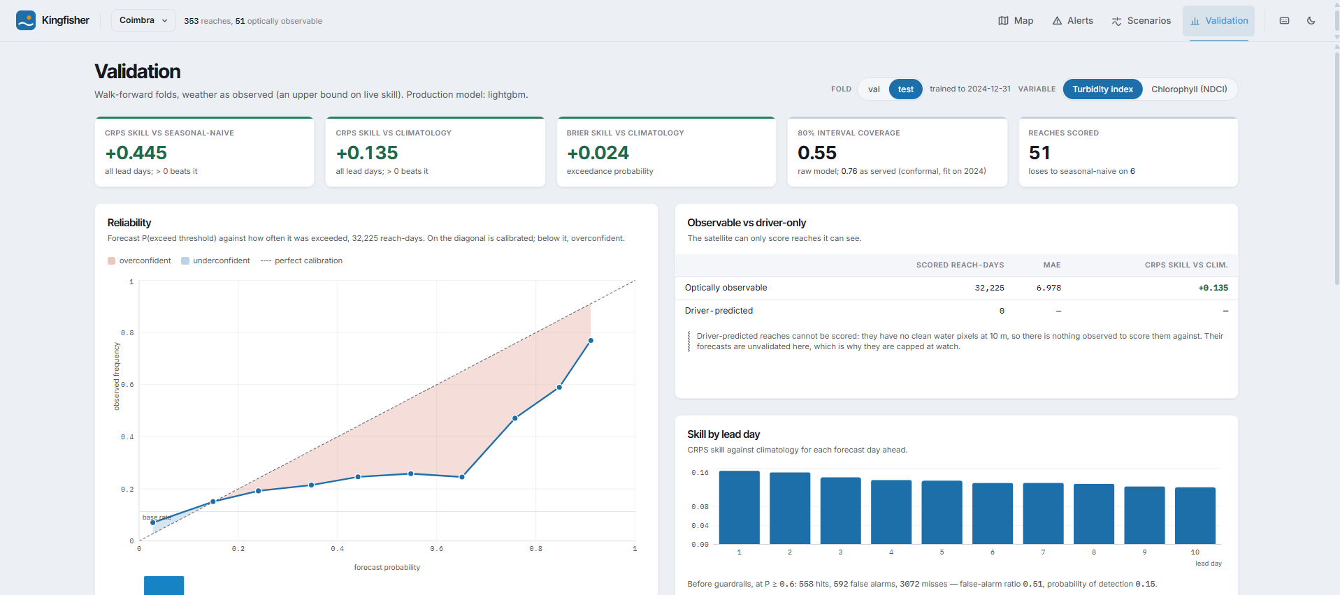
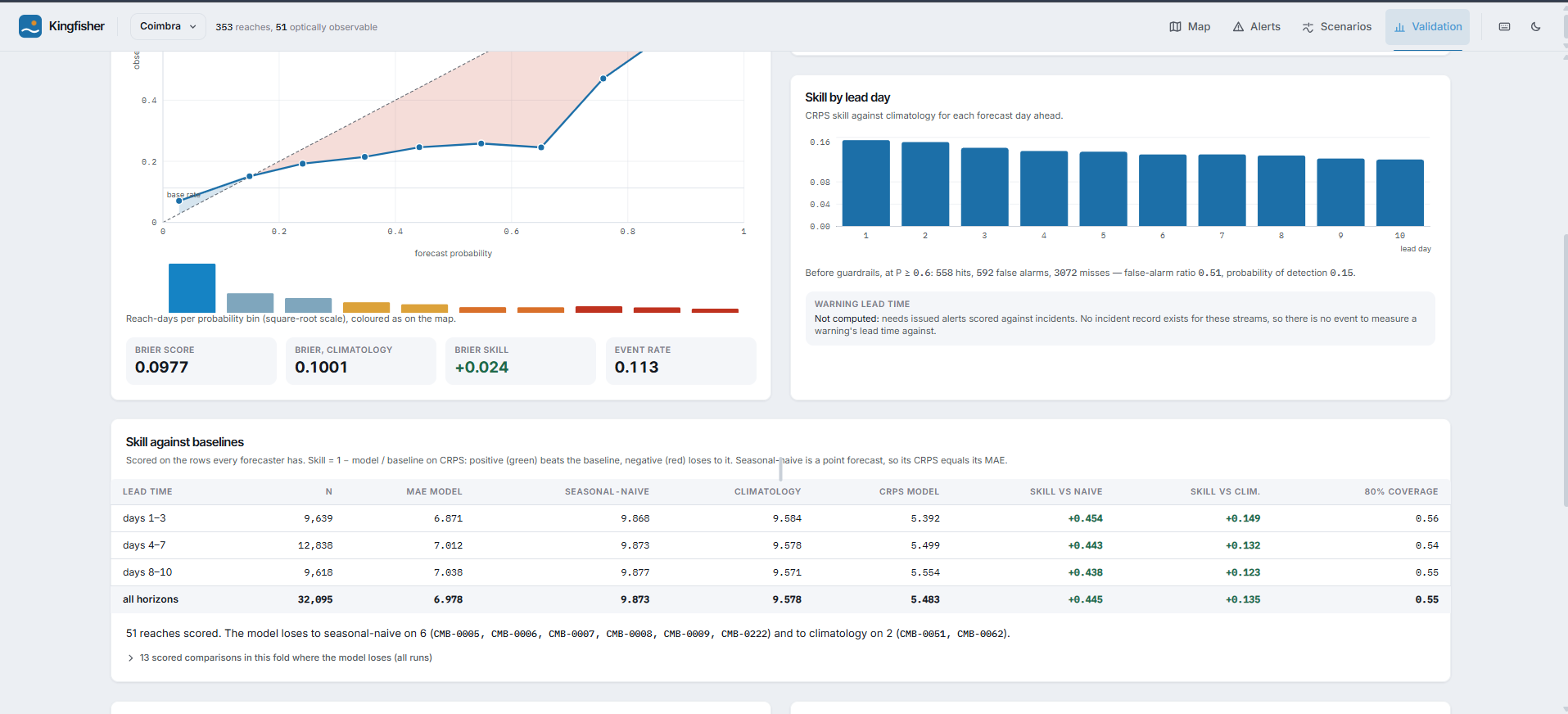
Turbidity validation shows mid-range overconfidence, while predictive skill remains consistent through the 10-day forecast horizon.
-
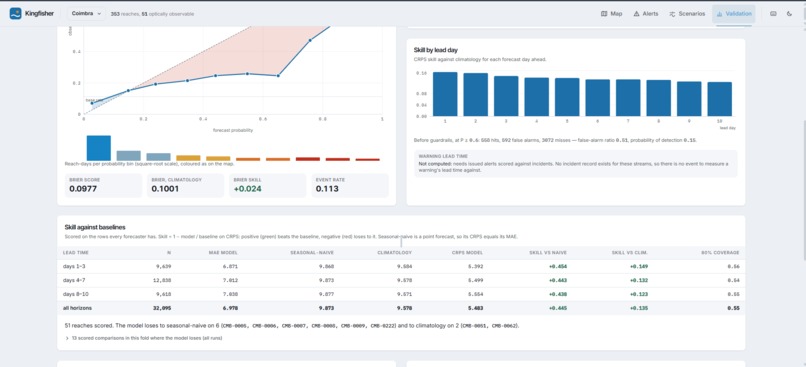
Turbidity Brier skill is only +0.024. Before guardrails, alerts at P≥0.6 have a false-alarm ratio of 0.51, reported as it is.
-
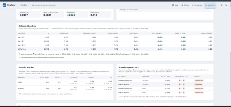
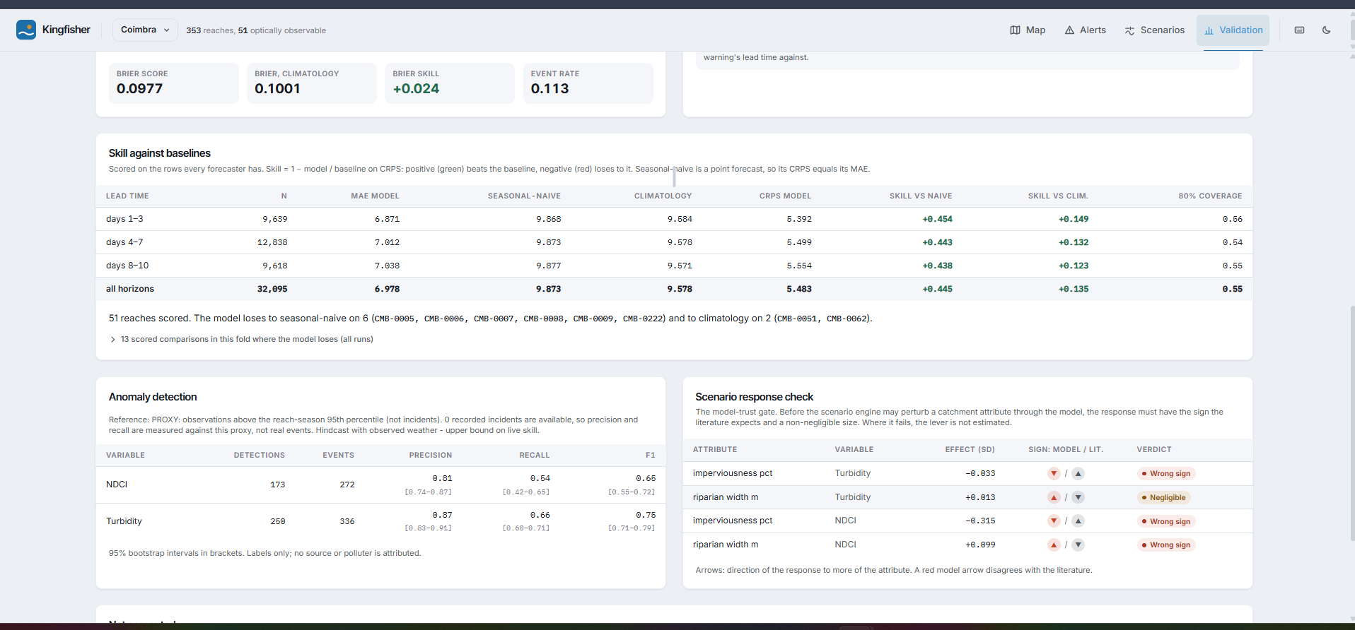
Turbidity underperforms seasonal-naive on 6 reaches; anomaly F1 of 0.75 is measured against a proxy, not real incidents.
-
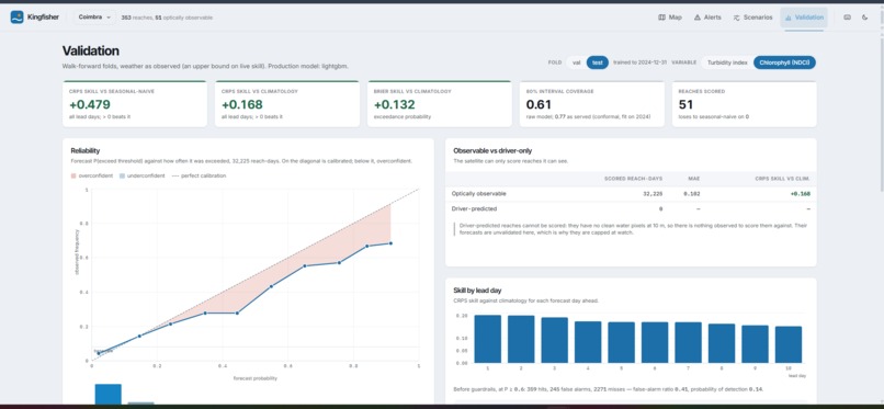
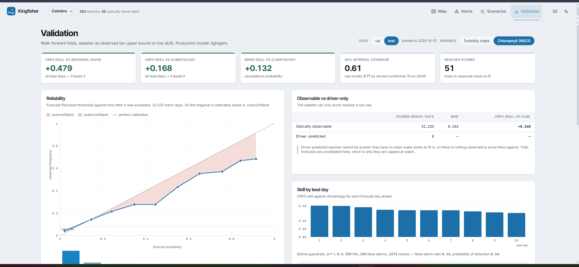
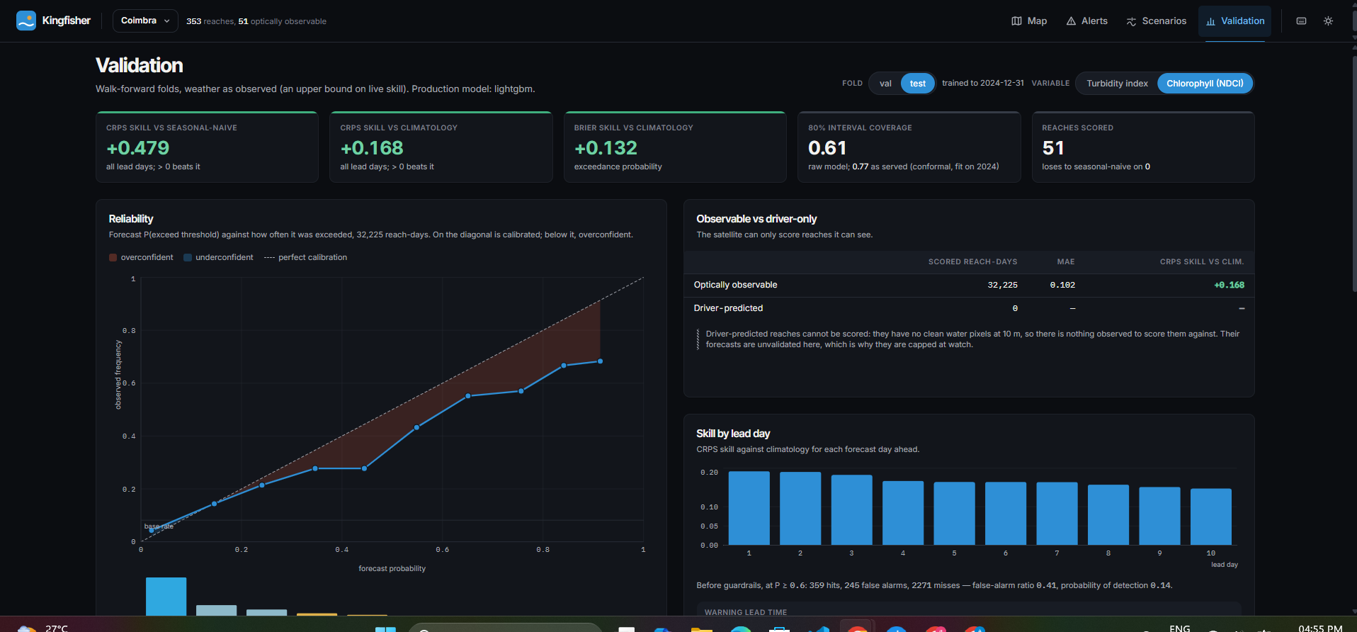
Chlorophyll validation: +0.479 CRPS skill vs seasonal-naive, reliability curve, and a note that driver-only reaches can't be scored.
-
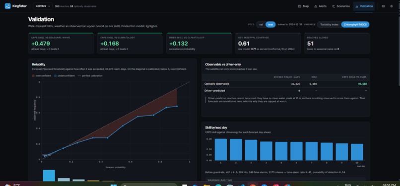
Chlorophyll validation in dark theme
-
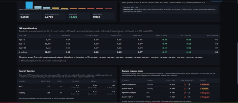
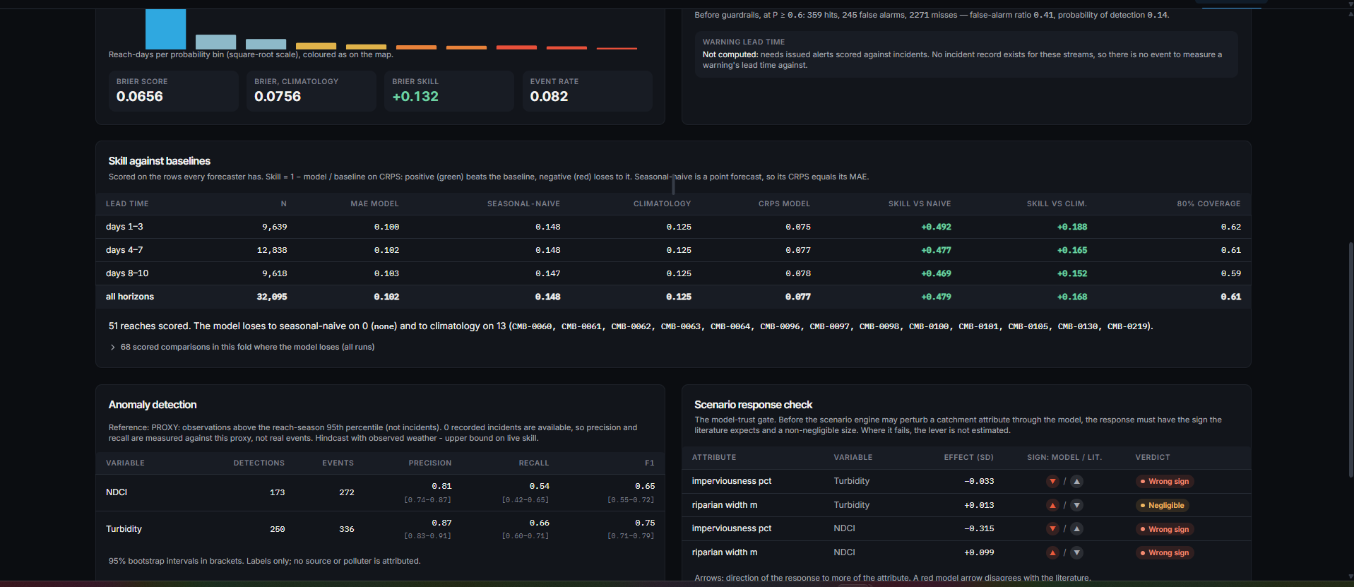
Chlorophyll skill vs baselines, anomaly precision/recall, and the scenario check where both catchment levers fail on sign or size.
Inspiration
Urban streams usually fail between sampling visits.
A dry spell ends with a hard storm, and in a few minutes weeks of road dust, sediment and contaminants wash off roofs and roads into the nearest stream. A storm overflow runs for an afternoon and is gone by the next morning. A warm, low-flow week lets algae bloom until oxygen crashes and fish die. All of these follow the weather. Professional monitoring follows a calendar, and citizen observation depends on whoever happens to walk past. A stream can fail on a Tuesday and be sampled a month later, when the water and the evidence have already moved on.
OneAquaHealth's own work across 100 urban stream sites in five European cities shows this gap. Pharmaceuticals were detected at 91% of monitored sites, and diatom deformities had to be used as an early-warning indicator because routine monitoring misses what happens between visits.
I realised the problem is not a lack of data. It is detection latency, plus the lack of any tool that tells a city what to change. A city water manager has no tool that answers three simple questions:
- Which reaches will be in trouble in the next ten days?
- Where is the next field visit worth the most?
- If I restore this riparian buffer or build that detention basin, how much less often will this stream exceed its normal range?
Track 6, Resilience Informatics, names this gap as a lack of predictive environmental tools and asks for predictive dashboards, alerts and resilience tools. Kingfisher is our answer, named after the bird that watches the water continuously and moves before anything else notices.
Kingfisher watches the water continuously, warns before the water turns, and shows what to change so it turns less often.
What it does
Kingfisher is an early-warning and resilience-planning system for urban stream networks. It runs on free, global data and needs no new sensors. It is built on three pillars.
1. Predict
For every reach (a 200 to 500 m segment) of a city's stream network, Kingfisher issues a 10-day forecast of a turbidity index and a chlorophyll index (NDCI). Each forecast has seven quantiles (P5, P10, P25, P50, P75, P90, P95), so every number comes with a prediction interval. Forecasts are issued daily on the ECMWF IFS 00 UTC run, which is the weather a live system would actually have.
2. Warn
Each reach is compared with its own seasonal normal: the 90th percentile of that reach's usable observations in that meteorological season, fitted only on the fitting period and never borrowed from a neighbour. From the calibrated forecast distribution, Kingfisher reads the probability that the reach will exceed that normal. The candidate alert then passes through five guardrails in a fixed order:
| Guardrail | Rule | Outcome |
|---|---|---|
| Staleness | Last usable evidence older than 21 days, or none at all | INSUFFICIENT_EVIDENCE |
| Drift | Recent residuals leave the calibration band | Suppressed |
| Confidence | Peak exceedance probability below 0.60 | Suppressed |
| Cooldown | An ALERT or WATCH for the same reach and variable in the last 72 hours | Suppressed |
| Observability | Reach not proven optically observable | Capped at WATCH |
Every alert records its basis: how the threshold was derived, the model version, the weather source, the top SHAP drivers on the peak day (in the target's units), and exposure context. Exposure means the schools, kindergartens, playgrounds, parks, healthcare sites, footways, cycleways, water access points and population within 250 m of the reach.
The system is also allowed to refuse. INSUFFICIENT_EVIDENCE is a first-class output. It is hatched on the map, counted in the metrics, and never turned into a low-confidence alert.
3. Adapt
A scenario workbench lets a planner click or lasso reaches on the map, choose interventions and their extent, and swipe between before and after. There are five literature-cited levers: riparian buffers, permeable paving, detention basins, street sweeping and green roofs. The output is the change in exceedance days over the window for each reach, with a widened interval, the cost in the source currency, and the citation shown beside the number. Every result is labelled a planning estimate, not a prediction.
Kingfisher also produces a prioritisation list ranking where the next field visit or citizen-science sample is worth the most:
$$\text{information value} = \text{forecast uncertainty} \times \text{predicted risk} \times \text{exposure weight}$$
It also runs anomaly detection, which separates readings the weather explains from readings it cannot, and a FHIR R4 export that turns an alert into a Bundle of Observation, Location and Device resources. With that export, an environmental early warning can enter a health information system in the format it already uses.
Two cities, one codebase
- Coimbra, Portugal (primary): 353 reaches.
- Pune, India: 312 reaches on the Mula-Mutha, in a south-west monsoon climate on a different continent. Pune was added with a YAML config file, a land-cover adapter and a post-monsoon riparian window.
The interface
A React and MapLibre dashboard with four views:
- Map: the network is coloured by exceedance probability. Hovering a reach shows its upstream catchment. Each reach opens a drawer with a fan chart, SHAP bars, a catchment card, an exposure list and an observability badge. A hydrograph rail scrubs the map through past observations and forecast days.
- Alerts: sorted by severity, with refusals shown alongside alerts.
- Scenario workbench: select reaches, apply levers, then compare before and after.
- Validation: reliability diagrams, a skill table that includes every loss, anomaly precision, recall and F1, and observable versus driver-only results, all served live from the evaluation output with its sha256 hash.
How I built it
The core idea: driver to state
Kingfisher combines two kinds of data, and neither is enough alone.
- Satellite data is continuous but shallow. Sentinel-2 is free, revisits every five days and goes back to 2015, but it only sees what water looks like. It will never see a pharmaceutical.
- Weather drives stream state and is available everywhere, every hour: rain intensity, dry spells, soil wetness, temperature and evaporation, both observed (ERA5) and forecast (ECMWF IFS).
So Kingfisher does not extrapolate a time series. It learns how the weather falling on a reach's upstream catchment, combined with that catchment's land cover, becomes the optical state of the reach. That choice pays off twice. Reaches too narrow for the satellite to see can still be forecast, and catchment attributes become model inputs that a planner can change, which is what makes the scenario engine possible.
L0: stream network and upstream catchments
OpenStreetMap waterways are noded at confluences, given a Strahler order and split into reaches with a 350 m target. Reaches below Strahler order 2 are dropped because no 10 m sensor can see them. Each reach outlet is snapped to a flow accumulation grid, and its upstream contributing catchment is delineated from precomputed flow direction. MERIT Hydro is the design source; the Copernicus DEM GLO-30 was used as a fallback while MERIT access was pending. We never derive flow direction from a raw DEM. Weather and land cover are aggregated over that catchment polygon, never over a circle drawn around the stream, because the catchment is the area that actually drains into the reach. Catchments that break monotonicity or snap off the network are flagged, not dropped.
L1: Sentinel-2 water indices
I used the Sentinel Hub Statistical API instead of downloading granules. At roughly 1 GB per granule across hundreds of scenes, downloading would have used up the whole timeline. Water pixels are those classified as water by both the Sentinel-2 scene classification and an MNDWI test, and water_pixel_count is stored on every reach-date.
- Turbidity index: the Nechad et al. single-band algorithm on the B4 red band, with ACOLITE coefficients for Sentinel-2 MSI. It is displayed as an index with no unit, because it is a reflectance proxy and not a nephelometric measurement.
- Chlorophyll index (Mishra and Mishra 2012):
$$\text{NDCI} = \frac{B5 - B4}{B5 + B4}$$
- Riparian NDVI: one composite window per reach-year (July in Coimbra; mid-October to mid-November in Pune, after the monsoon).
- Platform QA: a check for a level shift when Sentinel-2C entered service.
A missing reach-date is NULL with a quality flag (CLOUD, NO_WATER_PIXELS or OUT_OF_RANGE). It is never zero and never an unlabelled forward-fill. Every network response is cached to disk, keyed by its request parameters, before it reaches a DataFrame, so re-running the pipeline hits the network only once.
L2: weather drivers engineered for urban hydrology
Weather is queried at each catchment's centroid, snapped to the 0.1 degree ERA5-Land grid, which cut Coimbra's requests about 35-fold. The features follow urban stream physics:
- Antecedent precipitation index, for catchment wetness, with day t excluded and the value set to
NULLif any day in the window is missing, so a missing day is never read as a dry one:
$$\text{API}_k(t) = \sum_{i=1}^{k} P(t-i)\cdot 0.9^{\,i}, \qquad k \in \{7, 14, 30\}$$
- Antecedent dry days: consecutive days before day t with less than 1 mm of rain, for pollutant build-up on impervious surfaces.
- First-flush index, for a dry spell broken by an intense storm:
$$\text{first flush index} = \text{antecedent dry days} \times \text{peak hourly precipitation}$$
- Temperature times low flow, for conditions that favour algae, where the maximum is taken over training dates only so the test years cannot leak in:
$$\text{temp low flow index} = T_{\text{mean}} \times \left(1 - \frac{\text{API}_{14}}{\max_{\text{train}} \text{API}_{14}}\right)$$
- Soil moisture, reference evapotranspiration, seasonal harmonics, and an upstream state feature: the catchment-area-weighted latest observation of the direct upstream reaches. It lets information from a visible upstream reach flow down to a reach the satellite cannot see.
Training uses archive weather. I also rebuilt the ECMWF IFS 00 UTC runs as issued on every date since March 2024, so the model is scored on the forecast weather a live system would really have had (ASISSUED), not only on observed weather (ORACLE).
Static attributes (imperviousness, riparian width, riparian NDVI, road density, night-time light and population) come through a land-cover adapter chain: Copernicus CLMS where it exists, ESA WorldCover 10 m elsewhere. Every value records its source and any proxy flags.
The forecast model
A pooled LightGBM quantile regression, trained across all reaches with a reach embedding. Each reach has only about 500 usable timesteps, far too few for per-reach models. There are seven quantiles, and quantile crossings are rearranged and counted.
I trained two variants and report both:
- Variant A includes reach identity. It is the production forecaster.
- Variant B has no reach identity and powers scenarios. A model that knows which reach it is looking at can ignore the catchment attributes, so it cannot tell you what changing them would do. Variant A beats B by 7.6% (turbidity) and 18% (NDCI) in test CRPS. That is the price of a model that can run scenarios, and I publish it.
Validation is walk-forward with no shuffling: train through 2023 and validate on 2024; train through 2024 and test on 2025 to 2026. Leakage tests assert programmatically that no target-date information enters a training row.
Calibration
The raw quantile model was over-confident: its 80% interval covered only 55 to 61% of held-out observations. We applied split-conformal quantile regression (Romano, Patterson and Candès 2019), fitted only on the 2024 validation fold. The code raises TestFoldTouched if any other row reaches it. Live forecasts use the fit from as-issued weather. Served 80% interval coverage on the held-out test fold rose to 0.76 to 0.78.
The EA-LSTM challenger, and a gate fixed in advance
I trained an Entity-Aware LSTM with NeuralHydrology 1.13 (5 seeds by 2 targets, on a Colab T4) as a planned upgrade. Before the test fold was scored, I fixed a production gate: the challenger had to win at least 2 of 3 horizon buckets for both targets, with coverage no worse. It won 2 of 3 for NDCI, missing the coverage test by 0.00006, and 0 of 3 for turbidity. LightGBM stayed in production, and both models are reported side by side.
The scenario engine
A statistical model has no right to invent the effect of a green roof, so the engine keeps the model and the intervention physics apart.
- Every effect size lives in
config/intervention_coefficients.yaml, with magnitude, uncertainty range, applicability conditions, cost in source currency and full references. Every number must be claimed by a reference'ssupportslist, or the file refuses to load. Daylighting is listed asnot_quantifiedbecause the literature has no usable effect size. - A lever changes an input. For example, detention cuts peak hourly rainfall, which then changes the first-flush index.
- A binding response check moves each static attribute by plus or minus 1 SD on every held-out reach-day and compares the model's response with the sign the literature expects. The negligible cutoff (0.02 target SD) was fixed in config before the check first ran. Each lever and variable then takes one of three paths:
MODEL_PERTURBATION,LITERATURE_DIRECTorNOT_ESTIMABLE. - Output: exceedance days, computed as the sum of daily exceedance probabilities with a Poisson-binomial interval. The scenario interval is 1.5 times the larger of its own width and the baseline width, so it is always strictly wider than the baseline, and the caveat appears on screen rather than in a tooltip.
Engineering discipline
- Pure functions in
engine/: alerts, guardrails, scenarios, priorities, exposure, thresholds and probability code do no I/O at all, so every rule can be tested exhaustively without a server. - FastAPI with 16 API routes plus a health check, Pydantic models at every boundary, PostGIS 16 behind a repository
Protocol, and Alembic migrations. - Structured logging: every pipeline stage logs rows in, rows out, and rows dropped with the reason.
- About 500 tests. Guardrail tests break each guardrail on purpose and assert that the suite catches it. Leakage tests prove that calibration refuses test-fold rows and that assimilation ignores future observations. Quality-flag tests prove missing data never becomes zero. Feature fixtures are checked against hand-computed values. Scenario tests assert that every applied coefficient is cited and that every scenario interval is wider than its baseline. API contract tests check the Pydantic schemas.
- Frontend: React 19, TypeScript, Vite, MapLibre GL, Zustand, Tailwind and Recharts, with a dark-first "chart paper" visual language and a sediment colour ramp.
- Deployment: the whole system (PostGIS, API and frontend) is packaged into one Docker container and tested. Every API response the UI reads is then saved from that container, and the result is published as a static Hugging Face Space. The workbench replays 12 scenarios run by the real engine: each lever alone and all together, on the top 25 priority reaches.
A rule I never broke
No LLM computes a number. Every value in Kingfisher comes from a trained model or deterministic code.
Challenges I ran into
10 m pixels, 5 m streams
This constraint shaped the whole project. Sentinel-2's finest bands are 10 m, and urban streams are often 3 to 8 m wide. A pixel that straddles a stream mixes water, bank, road and roof, so its "turbidity" is meaningless. Our Day 1 observability gate showed the scale of the problem:
| Coimbra | Pune | |
|---|---|---|
| Reaches in the network | 353 | 312 |
| Optically observable | 51 (14%) | 59 (19%) |
| Driver-only (forecast, capped at WATCH) | 302 | 253 |
| Usable Sentinel-2 reach-dates | 14,141 | 16,069 |
| Lost to cloud | 19,761 | 17,549 |
| Lost to no water pixels | 4,303 | 4,580 |
| Rejected as out of range | 11 | 241 |
Only about one urban reach in six is visible from space at 10 m. Instead of hiding this, I report it as a finding about the limits of satellite monitoring for urban streams, and I designed the whole system around it. That is why the model is driver-based, why driver-only reaches are still forecast but never raised above WATCH, and why water_pixel_count is stored on every reach-date.
The model learned the wrong physics, and I said so
When I ran the response check in Coimbra, every static lever failed. Adding impervious cover lowered the forecast turbidity on 62 to 75% of reaches, for both LightGBM and the EA-LSTM. The cause is confounding. 37 of the 41 training reaches are large main-stem reaches of Strahler order 4 to 5, with a mean catchment of about 1,500 km² and mean imperviousness of only 8.6%, so the model learned a between-reach association, not the physical response.
It would have been easy to ship a scenario engine where every lever does something. I shipped one that says when the evidence cannot support a number:
- Permeable paving on turbidity takes the
LITERATURE_DIRECTpath in Coimbra. The model is bypassed, and the forecast is scaled by a cited suspended-solids removal of 0.82 (range 0.32 to 0.95), from the NWRM U3 guide citing DTI 2006 and SNIFFER 2004, multiplied by the share of impervious area treated. It is stated as an upper bound. On the top 25 priority reaches at 5 percentage points of treatment, it gives 12 to 30% fewer exceedance days on the 9 reaches with enough imperviousness to treat. - Green roofs and riparian buffers stay
NOT_ESTIMABLEin Coimbra. Their sources give no in-stream sediment figure, and I did not invent one. - Detention basins and street sweeping return honest, near-zero effects from the literature: a 0.3% cut in peak intensity for detention (Emerson et al. 2005, more than 100 basins at watershed scale) and a central value of 0 for sweeping (Selbig and Bannerman 2007).
In Pune, whose observable reaches span 0 to 69% imperviousness against Coimbra's 3 to 51%, the same check passed for imperviousness and turbidity, so paving and green roofs run through the model there. The same engine and the same rule reach different verdicts on different evidence, which is exactly why the check exists.
Calibration versus the alert floor
Chlorophyll probabilities came out well calibrated. Turbidity probabilities were over-confident in the 0.3 to 0.7 range: a forecast of 0.45 to 0.65 came true only about 25% of the time. With live forecast weather, raw turbidity Brier skill was negative 11.3% against climatology. Isotonic recalibration fixes the Brier score (to +4.0%), but then turbidity forecasts almost never reach the 0.60 alert floor: 3 flags in 14,506 held-out as-issued reach-forecasts. That floor was fixed before any of this was measured, and lowering it now would be tuning on the test set. So I serve conformal-calibrated quantiles, publish the result, and list the trade-off as open work.
Monsoon cloud in Pune
In Pune, cloud removes most observations exactly when rain-driven turbidity peaks (17,549 cloud-lost reach-dates against 16,069 usable). The model rarely sees the events it most needs to learn, so Pune turbidity only ties climatology. At the end of the monsoon, almost no reach has a cloud-free observation from the last 21 days, so on 23 September 2026 Kingfisher returned 576 INSUFFICIENT_EVIDENCE outcomes rather than alerting on stale evidence.
Hosting a geospatial ML system for free
Free Hugging Face Docker Spaces were not available to us, so I could not run a live server. We built the full system into one tested container, crawled every API response from it, and published a static snapshot that replays the real engine's outputs, with honest labelling wherever a live run is needed.
Data budgets and missing sources
MERIT Hydro access was pending, so Coimbra and Pune catchments run on the 30 m Copernicus DEM fallback, and monotonicity violations (21% of Coimbra catchments, 30% of Pune's) are flagged rather than dropped. The free Open-Meteo quota meant the as-issued weather backfill could not be run for Pune, so Pune's live intervals use the observed-weather calibration fit, and the record says so. No incident log existed for either city, so anomaly detection is scored against a clearly labelled proxy.
Accomplishments that I're proud of
Real forecast skill, at every lead time
On the held-out 2025 to 2026 test fold in Coimbra (never seen by any fit, threshold, calibration or gate decision), measured by CRPS skill:
$$\text{skill} = 1 - \frac{\mathrm{CRPS}{\mathrm{model}}}{\mathrm{CRPS}{\mathrm{baseline}}}$$
| Target | Weather | Lead 1-3 d | Lead 4-7 d | Lead 8-10 d |
|---|---|---|---|---|
| Turbidity vs seasonal-naive | observed | +45.4% | +44.3% | +43.8% |
| Turbidity vs seasonal-naive | as issued (live) | +44.1% | +41.6% | +34.4% |
| NDCI vs seasonal-naive | observed | +49.2% | +47.7% | +46.9% |
| NDCI vs seasonal-naive | as issued (live) | +46.0% | +43.6% | +41.0% |
| Turbidity vs climatology | observed | +14.9% | +13.2% | +12.3% |
| Turbidity vs climatology | as issued (live) | +13.6% | +9.3% | -1.2% |
| NDCI vs climatology | observed | +18.8% | +16.5% | +15.2% |
| NDCI vs climatology | as issued (live) | +11.5% | +8.7% | +7.1% |
Mean absolute error at lead 1 to 3 days: turbidity index 6.87 against 9.87 for seasonal-naive and 9.58 for climatology; NDCI 0.100 against 0.148 and 0.125. Skill decays gently with lead time, as a physically driven forecast should.
A system that knows when to stay quiet
The live run of 20 September 2026 in Coimbra, on the ECMWF run issued that morning, scored 706 candidates (353 reaches by 2 variables):
- 1 ALERT: CMB-0145 on the Rio Mondego, turbidity index, peak exceedance probability 0.62 between 21 and 30 September, with 1 school at 189 m, 5 footways and 8 cycleways within 250 m.
- 604
INSUFFICIENT_EVIDENCE: every driver-only reach, because none has a seasonal threshold of its own and Kingfisher will not borrow one. - 88 suppressed on confidence and 13 on drift (drift suppressions were 43 before the calibration fix).
Every run is recorded with its suppression counts, so "no alerts" is never confused with "no run".
Other results
- Calibrated intervals: served 80% coverage of 0.76 to 0.78, up from 0.55 to 0.61.
- Anomaly detection (hindcast, proxy reference, 2,000 bootstrap resamples): turbidity precision 0.87 (0.83 to 0.91), recall 0.66, F1 0.75; NDCI precision 0.81 (0.74 to 0.87), recall 0.54, F1 0.65.
- A second continent from a config file: Pune beats seasonal-naive by 44 to 47% on turbidity and 50 to 51% on NDCI, beats climatology on chlorophyll by 16 to 18% at every lead, and reaches 0.83 served interval coverage.
- Exposure mapping at city scale, summed over reach buffers (so overlapping buffers count twice): about 35,000 people, 40 schools and 25 playgrounds in Coimbra; 1.6 million people, 121 schools and 373 healthcare sites in Pune.
- An honest results table.
metrics.jsonlists all 130 cells (run by fold by variable by scope by metric) where a model loses to a baseline, and the README has a dedicated "Where it loses" section. The failed EA-LSTM gate and the failed intervention checks are reported as findings, not buried. - One Health interoperability: a FHIR R4 export that carries an environmental early warning into a health information system in its own format.
- About 500 tests, including a guardrail suite that breaks every guardrail on purpose.
- A live, public demo covering both cities.
What I learned
- Honesty is a feature. A system that can say "I do not know" (
INSUFFICIENT_EVIDENCE,NOT_ESTIMABLE, "not computed") earns more trust than one that always returns a number. The hardest part of building Kingfisher was keeping to that rule when a plausible number would have been easy to produce. - The physics has to shape the model. The mixed-pixel problem forced a driver-to-state design, and that design is also what made reach-scale forecasting of invisible reaches and the scenario engine possible.
- Hydrology beats geometry. Aggregating weather and land cover over the upstream contributing catchment, not a buffer, is what ties a reach to the land that feeds it.
- A good predictor is not automatically a good simulator. A model can forecast well and still learn the wrong sign for imperviousness. Checking a model's response against the literature before letting it size an intervention should be standard practice.
- Fix the rules before you see the answer. Deciding the EA-LSTM gate, the alert floor, the negligible cutoff and the calibration fold in advance protected the results from our own optimism.
- Evaluate on the weather you would really have. Scoring on as-issued ECMWF forecasts, not just observed weather, showed exactly where live skill fades (turbidity at 8 to 10 days).
- Calibration and alerting pull against each other. Better-calibrated probabilities can silence an alert system, and that trade-off belongs to the people who use the alerts, not to a quiet change made on the test set.
- Satellites have limits. Only 14 to 19% of an urban stream network is visible at 10 m. That is useful evidence for anyone designing a monitoring programme.
What's next for Kingfisher
- Ground-truth validation against SNIRH station series in Portugal and CPCB in India, which will let us score lead time and the false-alarm rate after guardrails, both currently listed as not computed.
- Resolve the turbidity calibration trade-off by re-choosing the alert floor on validation data for isotonic-recalibrated probabilities, with city partners in the loop.
- Downstream propagation of scenario effects through the reach topology, so a buffer upstream shows its benefit on every reach below it.
- MERIT Hydro catchments to replace the 30 m DEM fallback and clear the flagged monotonicity violations.
- Better land cover: true imperviousness layers and training reaches with a wider imperviousness range, so the model itself can learn to size static interventions.
- More cited coefficients for green roofs and riparian buffers, added only when the literature supplies a number.
- Cross-city transfer: scoring a Coimbra-trained model on Pune, and adding new cities with just a YAML file.
- A live hosted service with a daily scheduler in place of the frozen snapshot, plus complete as-issued weather history for Pune.
- Citizen-science integration, where volunteers sample the reaches on the prioritisation list and their samples flow back in as validation, working with OneAquaHealth Local Alliances.
- Climate scenarios that perturb the weather drivers for future rainfall and heat regimes.
Kingfisher does not predict disease, does not declare water safe or unsafe, and does not name polluters. It gives cities days of warning instead of weeks of hindsight, and an honest estimate of what to change.
Built With
- docker
- ecmwf
- esa-worldcover
- fastapi
- geopandas
- hugging-face
- lightgbm
- maplibre-gl
- neuralhydrology
- open-meteo
- openstreetmap
- postgis
- postgresql
- pydantic
- python
- pytorch
- rasterio
- react
- scikit-learn
- sentinel-2
- sentinel-hub
- shap
- tailwindcss
- typescript
- vite


Log in or sign up for Devpost to join the conversation.