
Checkout this interactive detailed tour of the site: https://app.supademo.com/demo/cmlxi0u5v0amf1435n2lqyk5j?utm_source=link
Without voiceover demo: https://youtu.be/gM7XDpd5big
Demo on Phone: https://youtu.be/Bsu0DACP7rI?si=iNpeoeP89R2PAOWB
Github Repo: https://github.com/Sadat41/HydroGrid
Site link: https://hydrogrid.app/
Our initial idea came from CIV E 321 (Principles of Environmental Modelling and Risk), a course from our 3rd year, and we realized the most annoying part of every assignment is just finding the data. Need precipitationn intensity for an IDF curve? That's Environment Canada. Flood zones? Alberta GIS portal. Drainage infrastructure? Edmonton Open Data. Property info for a site assessment? Another site entirely. We were spending more time copy-pasting URLs than actually doing analysis.
At one point we just said: what if we put all of this in one place and built the analysis tools on top of it? That's literally how HydroGrid started.
What it does
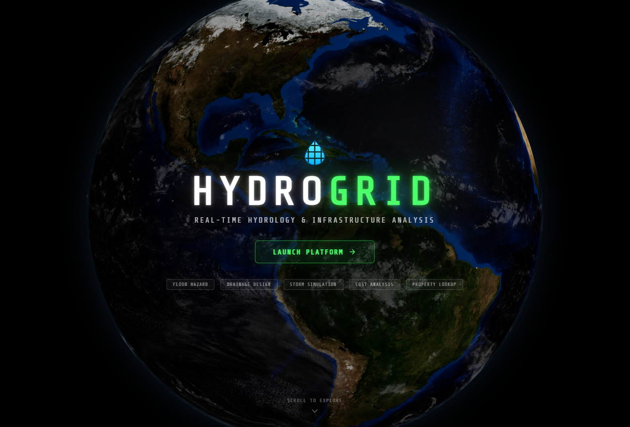
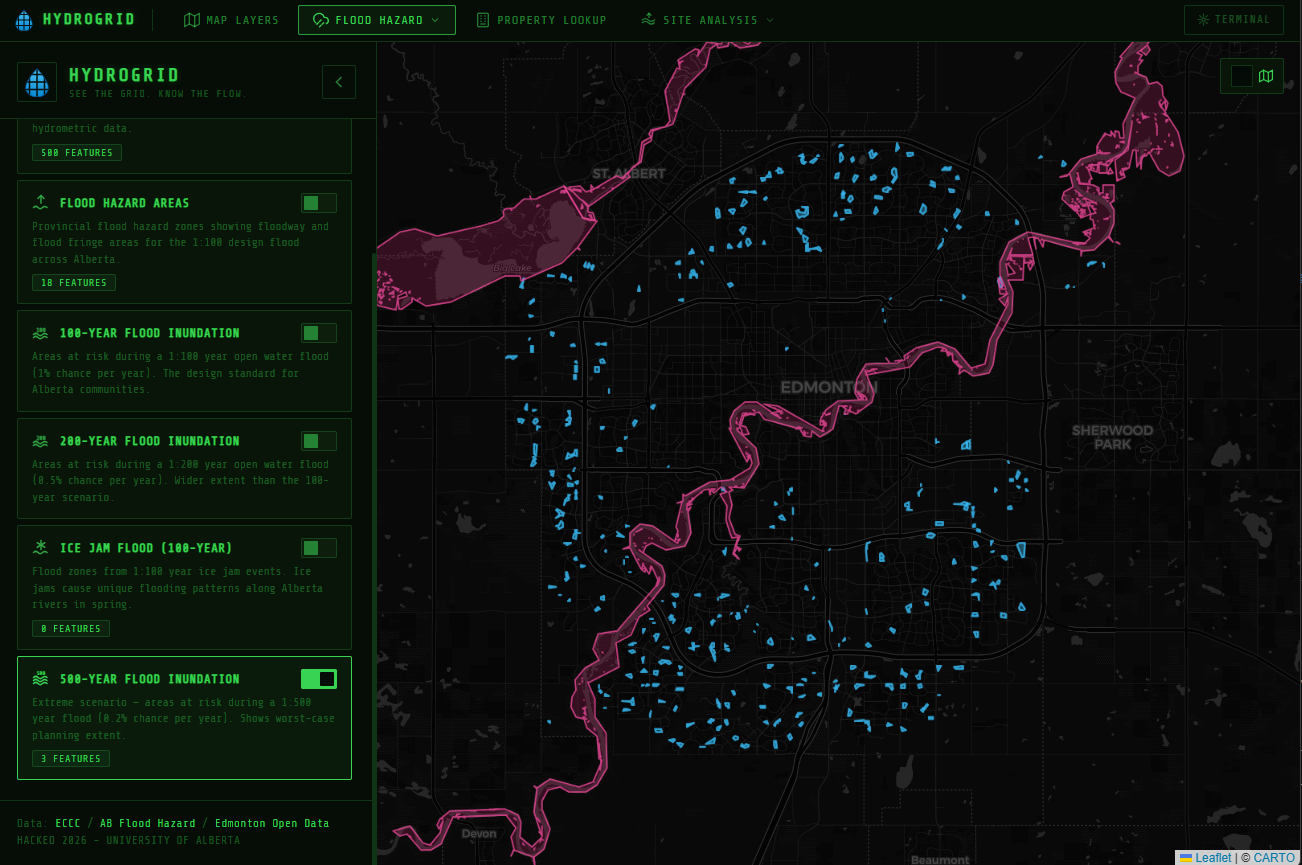
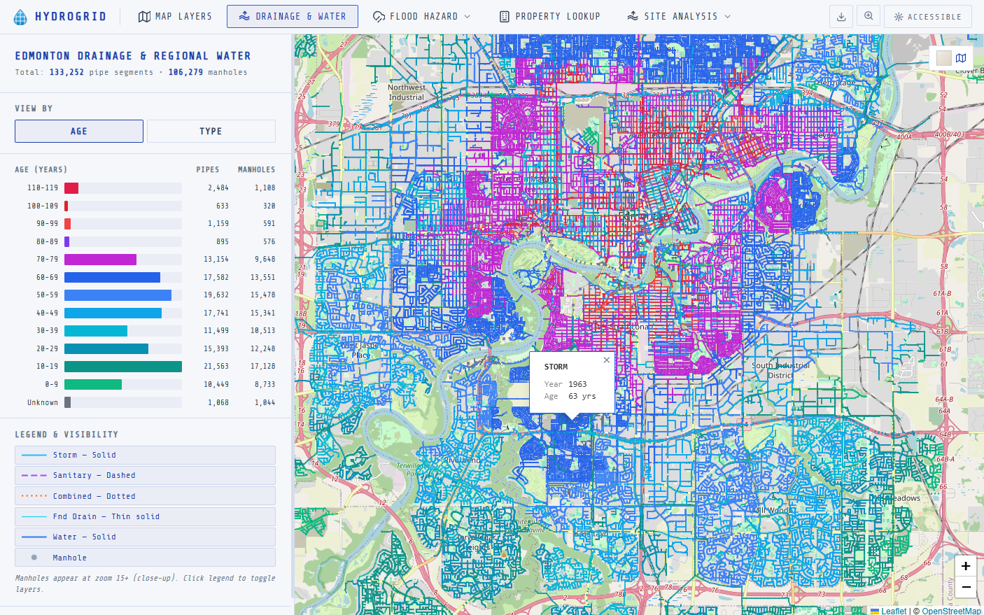
You open hydrogrid.app and get a live map with basically every hydrology-relevant dataset for Edmonton, layered on top of drainage networks, flood hazard zones (1:100, 1:200, 1:500 return periods), precipitation stations, river gauges, air quality monitors, property data, and building permits. Toggle whatever you need. Then on top of that:
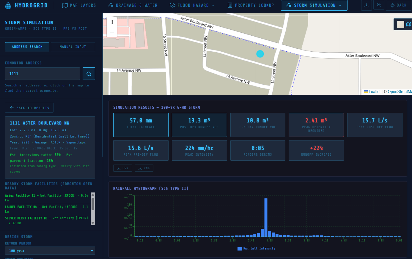
- Storm Simulation : pick a return period (2 to 100 yr) and storm duration, choose your soil type, set impervious fraction, and watch a full rainfall-runoff simulation play out step by step
- Site & Property Assessment : query any Edmonton parcel for lot size, zoning, building area, and overlay it against flood hazard zones
- Drainage Design Calculator : rational method pipe sizing with LID (Low-Impact Development) alternatives
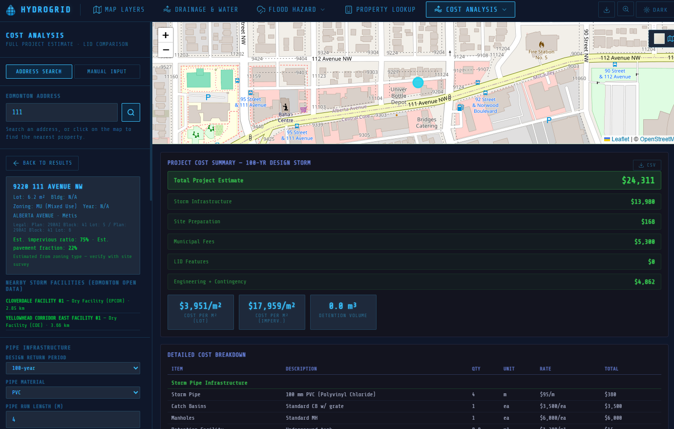
- Cost Estimator : full cost breakdown for stormwater infrastructure including excavation, pipe material selection, catch basins, manholes, and LID BMPs
Everything runs in the browser. No sign-up, no server, no install; just open the link and go.
How we built it
Stack
React 19 + TypeScript + Vite for the frontend. Leaflet.js for the interactive map with tiles from OpenStreetMap, CARTO, and Esri. Recharts for precipitation and flow timeseries. React Three Fiber + Three.js for the 3D landing page globe. All data comes from live API calls to Edmonton Open Data, Environment Canada, and Alberta's ArcGIS services; zero backend.
Government API Integration
The hardest part of the whole project was wrangling three completely different API formats into one consistent layer system. Edmonton Open Data uses Socrata (SODA), Environment Canada has its own REST format, and Alberta flood data lives on an ArcGIS FeatureServer.
For the ArcGIS layers (flood zones, drainage) we built a dynamic query builder that tiles requests to the viewport bounds and simplifies geometry at lower zoom levels to keep it fast:
  function buildArcGISUrl(
    baseEndpoint: string,
    bounds: LatLngBounds,
    zoom: number
  ): string {
    const sw = bounds.getSouthWest();
    const ne = bounds.getNorthEast();
    const bbox = `${sw.lng},${sw.lat},${ne.lng},${ne.lat}`;

    // fewer vertices at wider zooms, keeps rendering snappy
    const offset = 360 / (256 * Math.pow(2, zoom)) * 2;

    const params = new URLSearchParams({
      where: "1=1",
      outFields: "*",
      outSR: "4326",
      f: "geojson",
      resultRecordCount: "2000",
      geometry: bbox,
      geometryType: "esriGeometryEnvelope",
      inSR: "4326",
      spatialRel: "esriSpatialRelIntersects",
      maxAllowableOffset: offset.toFixed(6),
    });

    return `${baseEndpoint}/query?${params.toString()}`;
  }
Key endpoints we're calling:
  ┌───────────────────────────────────────────┬──────────────────────────────┬───────────┐
  │                  Dataset                  │            Source            │  Format   │
  ├───────────────────────────────────────────┼──────────────────────────────┼───────────┤
  │ Flood hazard zones (100/200/500-yr)       │ Alberta ArcGIS FeatureServer │ GeoJSON   │
  ├───────────────────────────────────────────┼──────────────────────────────┼───────────┤
  │ Property details, drainage infrastructure │ Edmonton Open Data (SODA)    │ JSON      │
  ├───────────────────────────────────────────┼──────────────────────────────┼───────────┤
  │ Precipitation stations, river gauges      │ Environment Canada API       │ JSON      │
  ├───────────────────────────────────────────┼──────────────────────────────┼───────────┤
  │ Basemap tiles                             │ CARTO / OSM / Esri           │ XYZ tiles │
  └───────────────────────────────────────────┴──────────────────────────────┴───────────┘
IDF Curves & Return Periods
This is straight out of lecture. An IDF (Intensity-Duration-Frequency) curve maps rainfall intensity (mm/hr) against storm duration for different return periods, the T-year storm means there's a 1/T annual probability of that event occurring or being exceeded.
We pulled IDF data for Edmonton City Centre (Climate ID 3012216) and implemented log-linear interpolation between standard durations, which is the standard approach when your design duration falls between tabulated values:
  // IDF intensities (mm/hr) for Edmonton - Climate ID 3012216
 const IDF: Record<number, Record<number, number>> = {
    2:   { 5:82,  10:56,  15:45,  30:30,  60:18,  120:11, 360:5.0, 1440:1.7 },
    5:   { 5:110, 10:76,  15:61,  30:41,  60:25,  120:15, 360:6.8, 1440:2.3 },
    10:  { 5:128, 10:89,  15:72,  30:48,  60:29,  120:18, 360:8.0, 1440:2.7 },
    25:  { 5:153, 10:107, 15:86,  30:58,  60:35,  120:21, 360:9.6, 1440:3.3 },
    50:  { 5:172, 10:121, 15:97,  30:66,  60:40,  120:24, 360:11,  1440:3.7 },
    100: { 5:192, 10:135, 15:109, 30:74,  60:44,  120:27, 360:12,  1440:4.2 },
  };
function getIntensity(rp: number, dur_min: number): number {
    const table = IDF[rp];
    const ds = Object.keys(table).map(Number).sort((a, b) => a - b);
    if (dur_min <= ds[0]) return table[ds[0]];
    if (dur_min >= ds[ds.length - 1]) return table[ds[ds.length - 1]];
    for (let j = 0; j < ds.length - 1; j++) {
      if (dur_min >= ds[j] && dur_min <= ds[j + 1]) {
        // Log-linear interpolation - standard for IDF curves (Bedient et al. 2019)
        const f = (Math.log(dur_min) - Math.log(ds[j]))
                 / (Math.log(ds[j + 1]) - Math.log(ds[j]));
        return Math.exp(
          Math.log(table[ds[j]]) + f * (Math.log(table[ds[j + 1]]) - Math.log(table[ds[j]]))
        );
      }
    }
    return 0;
  }
Storm Simulation: Green-Ampt + SCS Type II
The simulation engine is where most of the CIV E 321 content lives. For the rainfall distribution we use the SCS Type II 24-hour distribution (USDA NRCS TR-55), which is the standard design storm for inland continental climates like Edmonton. For infiltration we use the Green-Ampt model (Rawls, Brakensiek & Miller, 1983) which accounts for soil suction head and hydraulic conductivity:
$$f = K_s \left(1 + \frac{\psi \cdot M_d}{F}\right)$$
where \(K_s\) is saturated hydraulic conductivity, \({\psi}\) is the wetting front suction head, \(M_d\) is the available moisture deficit, and \(F\) is cumulative infiltration.
  // Green-Ampt soil parameters (Rawls, Brakensiek & Miller 1983)
  const GA_SOILS = {
    sand:        { Ks: 117.8, psi: 49.5,  theta_e: 0.437, theta_i: 0.10 },
    loam:        { Ks: 3.4,   psi: 88.9,  theta_e: 0.463, theta_i: 0.20 },
    siltLoam:    { Ks: 6.5,   psi: 166.8, theta_e: 0.501, theta_i: 0.22 },
    clay:        { Ks: 0.3,   psi: 316.3, theta_e: 0.475, theta_i: 0.30 }, // glacial till
    // ... (9 soil classes total)
  };

  // Per timestep - iterating over the SCS Type II hyetograph
  const fp = Ks * (1 + (psi * Md) / cumF);  // Green-Ampt infiltration capacity

  if (!ponded && intensity <= fp) {
    // All rain infiltrates - no runoff yet
    pervInf = rainStep;
    pervRunoff = 0;
  } else {
    ponded = true;
    pervInf = Math.min(fp * dt_hr, rainStep);
    pervRunoff = Math.max(0, rainStep - pervInf);
  }

  // Impervious fraction always contributes to runoff directly
  const runoffStep = pervRunoff * perviousFrac + rainStep * imperviousFrac;
This is the same infiltration excess (Hortonian) runoff mechanism we cover in 321, ponding occurs the moment rainfall intensity exceeds infiltration capacity, and runoff is the difference.
Drainage Design: Rational Method & Manning's Equation
The drainage calculator uses the Rational Method \(Q = C \cdot i \cdot A\) for peak flow estimation, with a composite runoff coefficient \(C\) built from land-cover fractions:
  function compositeC(buildingArea, pavementArea, lawnArea, totalArea, lid) {
    // Standard runoff coefficients (ASCE, City of Edmonton Design Standards)
    let roofC    = lid.greenRoof ? 0.40 : 0.95;
    let paveC    = lid.permeablePavement ? 0.30 : 0.90;
    const lawnC  = 0.25;

    let C = (roofC * buildingArea + paveC * pavementArea + lawnC * lawnArea) / totalArea;
    if (lid.rainGarden) C *= 0.85;  // ~15% first-flush capture reduction

    return Math.max(0.1, Math.min(C, 0.95));
  }
Time of concentration uses the Kirpich formula, then we look up intensity from the IDF table at that duration for the selected return period. Pipe sizing is Manning's equation for a circular pipe flowing full \(n = 0.013\) for PVC, \(S = 0.5%\):
\(D = \left(\frac{Q \cdot n \cdot 4^{5/3}}{\pi \cdot \sqrt{S}}\right)^{3/8}\)
  function requiredPipeDiameter(Q: number): number {
    const n = 0.013;   // PVC
    const S = 0.005;   // 0.5% slope
    const D_m = Math.pow((Q * n * 10.079) / (Math.PI * Math.sqrt(S)), 0.375);
    return D_m * 1000; // convert m → mm
  }
3D Globe: WebGL Atmosphere Shader
The landing page globe uses a custom GLSL atmosphere shader in Three.js, rim lighting via a Fresnel-like dot product in the fragment stage:
  // Fragment shader:atmosphere glow
  varying vec3 vNormal;
  void main() {
    float i = pow(0.65 - dot(vNormal, vec3(0, 0, 1)), 4.0);
    gl_FragColor = vec4(vec3(0.3, 0.6, 1.0) * i, i * 0.8);
  }
The biggest gotcha: a WebGL canvas running offscreen eats your entire CPU. We fixed it by using An IntersectionObserver to completely unmount the when the hero section scrolls out of view, not just hide it, actually remove it from the DOM:
  useEffect(() => {
    const obs = new IntersectionObserver(
      ([entry]) => setHeroHidden(!entry.isIntersecting),
      { threshold: 0.05 }
    );
    obs.observe(heroRef.current);
    return () => obs.disconnect();
  }, []);
  // In JSX - conditional render, not just display:none
  {!heroHidden && (
    <Canvas camera={{ position: [0, 0, 5.5], fov: 45 }} dpr={[1, 1.5]} ...>
      <GlobeScene />
    </Canvas>
  )}
Challenges we ran into
Government APIs are painful. The documentation is either missing or wrong half the time, the data formats are all over the place, and some endpoints just randomly stop responding. We also almost killed the browser trying to render a 3D globe and a scrolling page at the same time. Turns out if you leave a WebGL canvas running offscreen it eats your entire CPU. Had to figure out how to completely shut it down when you scroll past it. Also keeping things fast when you're pulling from like six different APIs at once with no backend to cache anything was tricky.
Accomplishments we're proud of
It actually works. We took data that's spread across like five different government websites and made it feel like one tool. The fact that anyone can just open a link and immediately start looking at real hydrology data without installing anything or making an account feels really good. Also the simulation and cost analysis stuff goes beyond just showing data on a map, it actually does useful engineering calculations which is what we wanted from the start.
What we learned
Real world data is messy. Like really messy. In class everything comes in nice clean CSV files but government APIs will give you missing fields, weird formatting, and schemas that change without warning. We also learned way more about browser performance than we ever expected to. And honestly just how much you can do with purely client side code these days without needing a server at all.
What's next for HydroGrid
Other cities. The way we built it, swapping in a different city's open data APIs isn't that hard so expanding beyond Edmonton is the obvious next step. We also want to add PDF report generation so you can export a full site assessment, better IDF curve analysis, and maybe some climate projection stuff. A mobile version for field use would be cool too.
Built With
- api
- carto
- claude
- css
- cursor
- esri
- github
- html
- leaflet.js
- nasa
- openstreetmap
- react
- react-leaflet
- recharts
- three.js
- typescript
- vite


Log in or sign up for Devpost to join the conversation.