Inspiration
Canadian farms face a difficult irrigation problem: crop water demand changes with weather, while soil water storage varies by field. A fixed watering schedule cannot account for tomorrow’s rainfall, a crop’s growth stage, or the amount of water a particular irrigation system can deliver. We built Hydrigate to turn public environmental data into a field-specific, explainable irrigation plan.
What it does
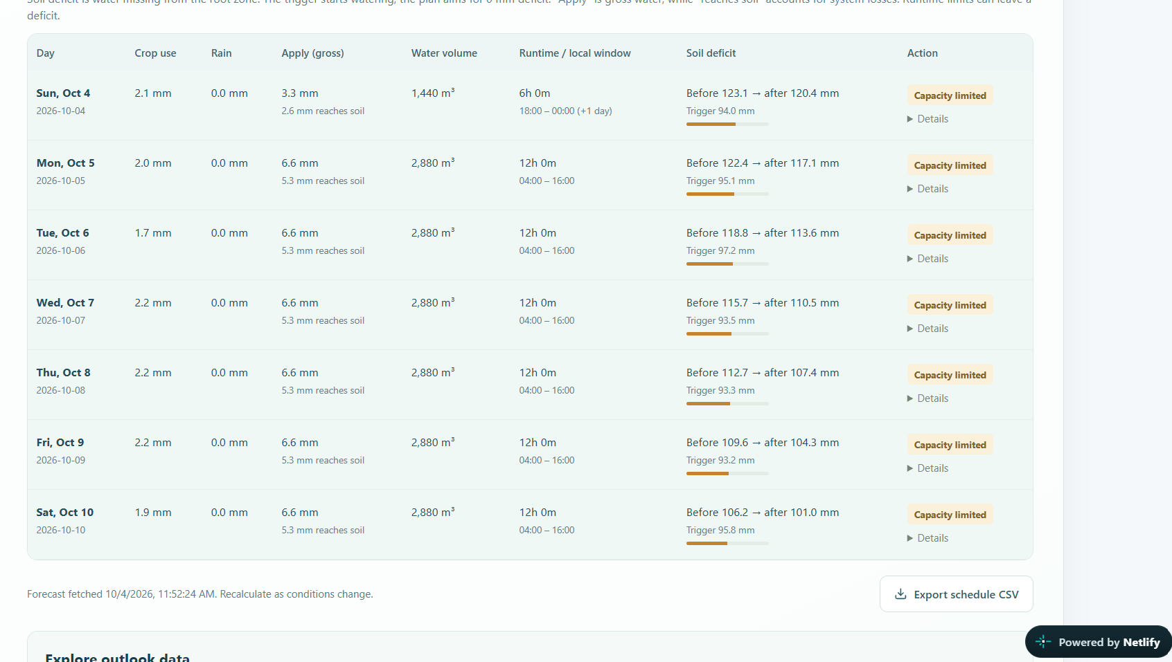
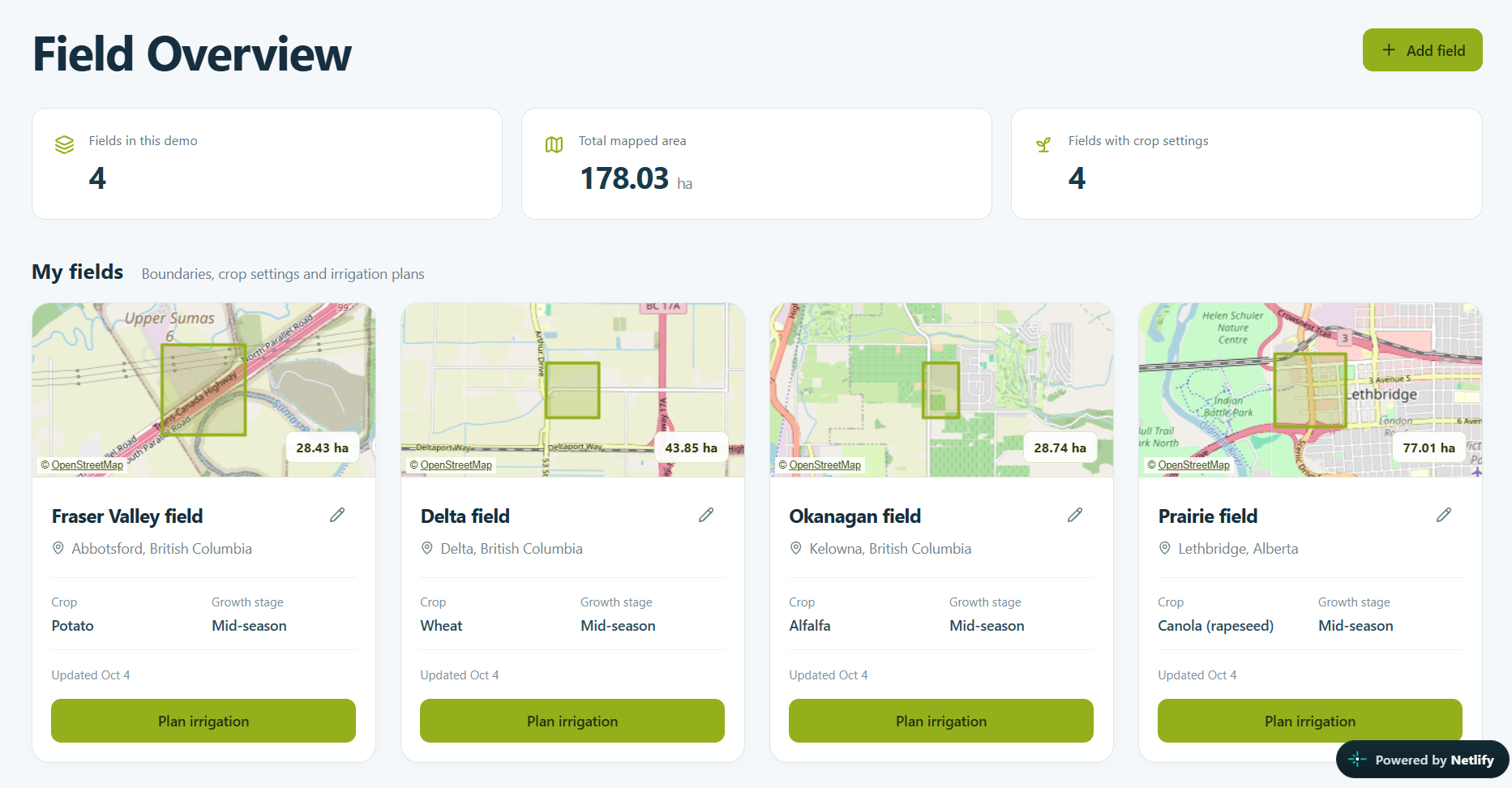
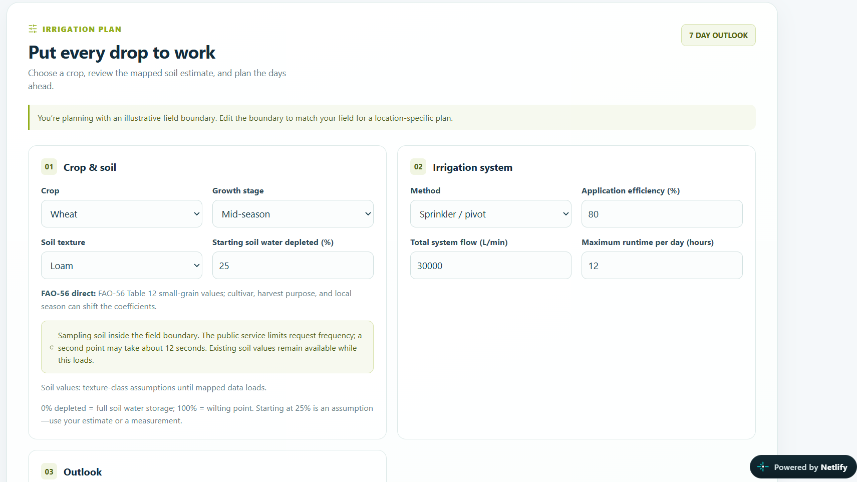
A farmer maps a field, chooses a crop and growth stage, and enters their irrigation system’s capacity. Hydrigate estimates how much water the root zone can store, predicts its daily depletion, and generates a 2–14 day schedule showing when to irrigate, how much to apply, and how long the system must run. Farmers can inspect graphs, download daily data, and override estimated inputs when they have better local measurements.
Data used
- Farmer’s field and equipment: Polygon coordinates; crop and growth stage; estimated starting soil-water depletion; irrigation method; application efficiency; total flow in litres per minute; maximum daily runtime; and the fraction of rainfall assumed to enter the root zone. Estimated crop and soil properties remain editable.
- Open-Meteo forecast [6]: Daily FAO reference evapotranspiration (ET_0), total precipitation, rain, showers, minimum and maximum air temperature, and maximum wind speed. Hourly temperature, wind, rain and showers are used to screen sprinkler watering windows. Total precipitation is shown to the farmer, while liquid rain plus showers enters the soil-water balance; forecast snowfall is not treated as immediate liquid irrigation water. Open-Meteo has 30+ weather models globally and it uses ML with multiple historical datasets that span from 1940 for accurate predictions with a resolution of 1km.
- Mapped soil: SoilGrids supplies sand, silt, clay and soil organic carbon estimates at up to two points inside the polygon, across depth layers from 0–5 cm to 100–200 cm. Hydrigate weights the layers over the selected root depth and uses the Saxton–Rawls pedotransfer equations to estimate field capacity and permanent wilting point.
- Crop properties: A library of 24 Canadian-relevant crops supplies growth-stage crop coefficients (K_c), estimated effective root depth (Z_r), and allowable depletion fraction (p). Values come from FAO-56 where available; related crop-class proxies are labelled as estimates.
- Farmer inputs: Crop and stage, starting soil-water depletion, irrigation method, application efficiency, total system flow, maximum daily runtime, forecast length, and an editable fraction of rainfall assumed to enter the root zone. Soil and crop defaults can also be changed.
How I built it
1. Measure the field. Longitude and latitude are projected into local metre-based coordinates. The shoelace formula then calculates polygon area:
$$ A=\frac{1}{2}\left|\sum_{i=1}^{n} (x_i y_{i+1}-x_{i+1}y_i)\right|. $$
Area matters because one millimetre of water over one square metre equals one litre. It converts a soil-water depth into the total volume a pump must supply.
2. Estimate how much water the soil can hold. SoilGrids provides mapped texture and organic carbon, not direct measurements of water storage. The Saxton–Rawls pedotransfer equations [4] use those properties to estimate volumetric water content at field capacity (\theta_{FC}) and permanent wilting point (\theta_{WP}). Hydrigate combines estimates across the root-zone depth. Total available water is
$$ TAW=1000(\theta_{FC}-\theta_{WP})Z_r, $$
where (Z_r) is root depth in metres and (TAW) is in millimetres. Field capacity is the approximate upper storage limit after excess water drains; wilting point is the lower limit beyond which the model treats water as unavailable to the crop. For example, a 0.6 m root zone with (\theta_{FC}=0.28) and (\theta_{WP}=0.14) has (TAW=84) mm. This is an illustrative calculation, not a measurement of a submitted field.
3. Estimate crop demand. Open-Meteo supplies (ET_0), the forecast water use of a reference crop. Hydrigate applies the selected crop and growth-stage coefficient from FAO-56 [3]:
$$ ET_{c,t}=K_cET_{0,t}. $$
Thus, a forecast (ET_0) of 4 mm/day and (K_c=1.15) imply an estimated crop demand of 4.6 mm/day. (ET_c) is a planning estimate under the crop-coefficient method, not a measurement of actual water loss from that field.
4. Update the daily soil-water balance. Hydrigate tracks depletion (D_t): zero means the modelled root zone is at field capacity; a larger number means more water has been removed. Each day, crop demand raises depletion and effective liquid rain lowers it:
$$ D_t^{*}=\operatorname{clip} \left(D_t+ET_{c,t}-P_{\mathrm{eff},t},\,0,\,TAW\right). $$
For example, 4.6 mm of crop demand and 1 mm of effective rain increase depletion by 3.6 mm. The bounds stop the daily “bucket” from storing more than field capacity or losing more than its total available water. Surplus rain is treated as drainage; the prototype does not calculate a soil-specific deep-percolation rate.
5. Decide when to irrigate. FAO-56 adjusts a crop’s allowable depletion fraction according to daily crop demand [3]:
$$ p_t=\operatorname{clip} \left(p_{\mathrm{base}}+0.04(5-ET_{c,t}),\,0.10,\,0.80\right), \qquad RAW_t=p_tTAW. $$
(RAW_t) is the baseline amount of depletion permitted before the model expects increasing crop-water stress. Hydrigate adds its own early-planning rule, triggering irrigation at
$$ T_t=\max(0,\;RAW_t-0.20TAW). $$
Because depletion rises as soil dries, this lower trigger starts planning before depletion reaches the FAO-56 baseline. The 20% buffer is a Hydrigate design assumption, not an FAO-56 prescription.
6. Give an actionable recommendation. Once triggered, the plan aims to replace the modelled depletion. If application efficiency is (\eta), gross irrigation must exceed the water intended to reach the root zone:
$$ I_{\mathrm{gross}}=\frac{I_{\mathrm{net}}}{\eta}, \qquad V=I_{\mathrm{gross}}A, \qquad t_{\mathrm{run}}=\frac{V}{Q}, $$
where (V) is litres and (Q) is system flow in litres per minute. Hydrigate caps runtime by the farmer’s daily limit and the available local-day or suitable weather window. It holds irrigation on freezing days. Its sprinkler-window rules check hourly wind, temperature and rain, and if a system cannot complete a refill, the remaining depletion carries into the next day.
Challenges we ran into
I had to learn and do a significant amount of research on the hydrologic and irrigation. Particularly, hydrigate relies on a physically consistent water balance at its core, so I had to cross-check and ensure it was working properly.
Estimating root-zone storage from the soil maps also posed problems. SoilGrids reports texture and organic carbon across several depths, but sometimes has missing values. The layers of the soil had to be combined over the crop’s root depth, and the Saxton–Rawls equations were applied to estimate field capacity and wilting point. There were issues with unit consistency , but that was also fixed.
Accomplishments that I'm proud of
Hydrigate integrates geospatial measurement, soil-water physics, crop-stage demand, live evapotranspiration and precipitation forecasts, and the farmers' constraints into a single analytical model. Essentially, it captures all the physics of irrigation. This is far more useful to farmers than any weather forecast because very significant factors like evapotranspiration aren't accounted for and even the raw data isn't accessible in a user-friendly manner for them. With Hydrigate, farmers can examine graphs and export the underlying forecast of all the data that is used for the soil- water balance.
What I learned
I learnt that irrigation is a lot more complex than it seems. There are complex physical systems that can impact crop health, and these must be accounted for in order to make agriculture more efficient and sustainable.
What's next for Hydrigate
I want to calibrate the model against soil-moisture sensors and recorded irrigation, quantify forecast uncertainty, and improve estimates of runoff and deep drainage for different soils. Those steps would make the model much more accurate. I hope this can help farmers.
References
[1] Food and Agriculture Organization of the United Nations, The State of the World's Land and Water Resources for Food and Agriculture—Systems at Breaking Point. Rome, Italy: FAO, 2021. doi: 10.4060/cb7654en.
[2] World Wildlife Fund, “Water scarcity.” [Online]. Available: https://www.worldwildlife.org/threats/water-scarcity. Accessed: Oct. 4, 2026.
[3] R. G. Allen, L. S. Pereira, D. Raes, and M. Smith, Crop Evapotranspiration: Guidelines for Computing Crop Water Requirements, FAO Irrigation and Drainage Paper 56. Rome, Italy: FAO, 1998. [Online]. Available: https://www.fao.org/4/X0490E/X0490E00.htm.
[4] K. E. Saxton and W. J. Rawls, “Soil water characteristic estimates by texture and organic matter for hydrologic solutions,” Soil Science Society of America Journal, vol. 70, no. 5, pp. 1569–1578, 2006, doi: 10.2136/sssaj2005.0117.
[5] L. Poggio et al., “SoilGrids 2.0: Producing soil information for the globe with quantified spatial uncertainty,” SOIL, vol. 7, pp. 217–240, 2021, doi: 10.5194/soil-7-217-2021.
[6] Open-Meteo, “Weather Forecast API documentation.” [Online]. Available: https://open-meteo.com/en/docs. Accessed: Oct. 4, 2026.
Built With
- leaflet.js
- netlify
- next.js
- nvidia-api
- open-meteo
- openstreetmap
- react
- soilgrids
- typescript

Log in or sign up for Devpost to join the conversation.