GRIME (Garbage River Interception & Modeling Engine)

Grime Logo
Dashboard
Landing Page

Inspiration

When Abhav visited his dad's small river town in India, he noticed a problem that stopped him mid-step. The river that had supported the community for years, the one his dad grew up swimming in and families still washed clothes with, was choked with pollution. Plastic waste bobbed against the bank, with the current carrying it farther into town. And this film of waste stretched downstream as far as he could see.

The locals weren't ignoring it, but they couldn't fix it either. The river was too wide to entirely block, the current too strong for makeshift barriers, and no one could tell them where intervention would actually make a difference. Nets that were tried downstream tore within weeks, while those upstream sat in the wrong spots entirely.

That experience stuck with him, and data shows how this problem isn't just localized: over 1,500 rivers across the world are responsible for 80% of all ocean-bound plastic, most of them too irregular for conventional netting. The question then became:

If we can't net every river, and the nets you do place keep failing, how do you decide where your limited resources will capture the most plastic?

Today, we introduce GRIME: A solution to that very question. Not bigger nets or more nets, but the right ones in the right places. GRIME extends the methodology of the WaterGate model (Cheng, Anand, Rose, 2023)[^1], which scored flood-prone locations on three parameters: catchment area, runoff coefficient, and discharge. GRIME redirects that hydrological framework toward trash accumulation prediction and expands it from 3 to 28 parameters across 6 families, adding feasibility constraints, environmental justice weighting, and a two-level scoring architecture.

What it does

GRIME is a multi-parameter optimization engine that identifies the best locations to deploy trash interception nets in waterways, anywhere on Earth. Rather than guessing where to put nets or relying on expensive manual surveys, GRIME evaluates every candidate site using 28 geospatial parameters organized into 6 parameter families, which aggregate into 4 interpretable sub-scores:

Generation: Is trash entering here?
Flow: How does water move it?
Impact: What will happen downstream?
Feasibility: Can we even install a net?

These combine into a single composite score from 0 to 100 via a two-level weighted architecture (detailed in the scoring section below). Sites where deployment is physically impossible, because of channels too wide to span, currents too fast for anchoring, or confirmed private land, are eliminated by hard gates before scoring begins. The model also explicitly weights environmental justice through EPA EJSCREEN data, prioritizing sites that serve overburdened communities.

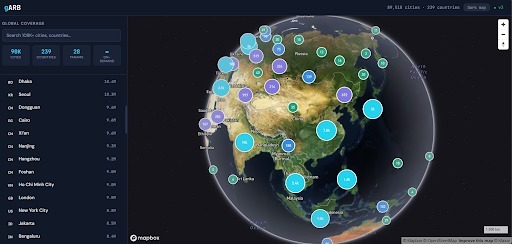
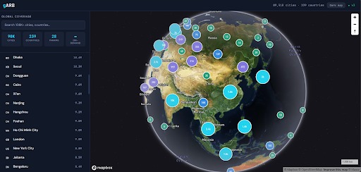
The system works in two modes. The research pipeline ingests real 10m elevation data from USGS 3DEP, runs a full computational hydrology pipeline to extract stream networks, then scores every candidate point using live data from six free, keyless federal APIs (USGS, EPA, Census). The interactive dashboard lets anyone click on any of 108,772 cities across 240 countries, fetches real waterway geometry from OpenStreetMap, generates and scores net placements client-side, and renders color-coded results on a Mapbox map in under 5 seconds.

The output is a ranked list of deployment sites with sub-score breakdowns and parameter evidence for each one.

How we built it

Hydrological Pipeline

We built a DEM-based hydrology engine using pysheds that takes raw 10m elevation data from USGS 3DEP and produces a complete stream network. The pipeline fills pits, resolves depressions and flats, computes D8 flow direction, runs flow accumulation, and extracts stream geometries at a configurable threshold (500 cells $= 0.05 \text{ km}^2$). Candidate net sites are then generated every 200m along extracted streams.

Raw vs Conditioned DEM Left: raw DEM with artifacts and noise. Right: conditioned DEM after pit-filling and smoothing — the input to our flow direction pipeline.

D8 flow direction field over synthetic terrain. Each arrow points to whichever of the 8 neighboring cells is lowest — the foundation of our stream network extraction.

Flow Accumulation Surface Flow accumulation on log scale for Durham, NC. Ridgelines show near-zero accumulation; valley channels spike to high values — exactly where streams form.

Parameter Computation

Each candidate is evaluated on 28 parameters pulled from six federal APIs (USGS NWIS, EPA ECHO, EPA EJSCREEN, EPA TRI, Census ACS, USGS PAD-US). Flow velocity is estimated using Manning's equation applied to DEM-derived slope and channel geometry:

$$V = \frac{1}{n} \cdot R^{2/3} \cdot S^{1/2}$$

where n is Manning's roughness coefficient (selected by channel type, ranging from 0.015 for concrete-lined urban channels to 0.070 for sluggish weedy ones), R is the hydraulic radius in meters, and S is the channel slope.

$$R = \frac{W \times D}{W + 2D}$$

where W is channel width and D ≈ 0.3W (bankfull approximation). A continuity cross-check is performed against USGS gauge data, and the final velocity estimate is the geometric mean:

$$V_{\text{final}} = \sqrt{V_{\text{Manning}} \cdot V_{\text{continuity}}}$$

This hedges against errors in either the DEM slope (which can be noisy at 10m resolution) or the rectangular channel assumption.

Manning's Equation Surface Manning's equation as a function of slope and roughness coefficient at fixed hydraulic radius $R = 0.5$ m. Steep, smooth channels (front-right) yield the highest velocities.

Proximity-based parameters use a Cauchy kernel for inverse-distance scoring:

$$\text{score} = \sum_{i=1}^{N} \frac{1}{1 + (d_i / h)^2}$$

where d_i is the distance to source i and h is the half-decay distance (500m default). Drinking water intake proximity uses an exponential decay instead — score = Σ exp(−d_i / 10) — giving intakes within 5km a weight of ≈ 0.61 and those within 1km a weight of ≈ 0.90.

Scoring Architecture

We designed a two-level weighted scoring system: 28 parameters aggregate into 4 interpretable sub-scores, which combine via a second weight layer into the composite. This structure has a specific advantage. A city planner can look at a candidate and immediately see "high generation, low feasibility" without needing to parse 28 individual numbers.

Generation Sub-Score Surface Generation sub-score as a function of population density and impervious surface coverage. Dense, paved urban areas (top-right) score highest.

Feasibility Score Surface Feasibility score across channel width and flow velocity. The green plateau is the viable installation zone — channels narrow enough to span and fast enough to carry debris, but not so fast that anchoring fails.

Composite Score Surface Composite score as Generation and Impact vary, with Flow and Feasibility held fixed. The linear response reflects the weighted architecture — no black-box nonlinearities.

To test whether top-ranked sites are robust to our specific weight choices, the system performs Monte Carlo sensitivity analysis. We sample 50 perturbed weight vectors from a Dirichlet distribution:

$$\boldsymbol{\omega}' \sim \text{Dir}(\boldsymbol{\alpha}), \quad \boldsymbol{\alpha} = 10 \times [0.30,\ 0.25,\ 0.30,\ 0.15]$$

The scaling factor of 10 controls perturbation magnitude, concentrating samples near the baseline weights. For each perturbation, composite scores are recomputed and the top 5 sites are recorded. A site's robustness is the percentage of perturbations where it appears in the top 5. A site with 90% robustness is a confident recommendation. A site at 30% is sensitive to weight assumptions and should be scrutinized.

Robustness Distribution Robustness score distribution across all candidate sites. Most sites cluster near zero — genuinely good placements are rare, which is exactly the point.

Rank stability heatmap across 50 Dirichlet perturbations. Top-ranked sites (top rows, green) hold their position. Lower-ranked sites (bottom rows, red) shift substantially — flagged for scrutiny.

Dashboard

The frontend is a single index.html file using Mapbox GL JS with a 7MB places database. Clicking any city fires an Overpass API query for real waterway geometry, runs a three-phase placement algorithm entirely client-side (constraint satisfaction, full scoring, then population-scaled risk-percentile filtering), and renders results in under 5 seconds. Dashboard scores are approximate; the Python pipeline is the authoritative scoring implementation.

Tech Stack

Component	Technology
Core language	Python
Hydrology	pysheds, py3dep
Geospatial	GeoPandas, Shapely, rasterio
Math	NumPy
API server	FastAPI, uvicorn
Frontend map	Mapbox GL JS
Waterway data	OpenStreetMap Overpass API
Federal data	USGS, EPA, Census (all free, keyless)

Challenges we ran into

pysheds on Windows. The DEM hydrology pipeline depends on pysheds, rasterio, and fiona, all of which have C dependencies that frequently fail to compile on Windows. We solved it by building the dashboard as a fully independent client-side system that bypasses pysheds entirely, using OSM waterway data and simplified scoring instead.

No ground truth. There is no public dataset of correct trash net placements. Every weight in the model is set by informed heuristic and literature, not optimization. We partially addressed this with the Dirichlet sensitivity analysis: if a site ranks highly across 50 different weight perturbations, it's probably a genuinely good location regardless of our specific weight choices.

OSM data coverage is uneven. OpenStreetMap has excellent waterway data in the US and Europe but highly variable coverage in developing nations, exactly the places that need trash interception most.

Channel width estimation. Fewer than 5% of OSM waterways have width tags. We built a heuristic estimator based on waterway type, but it's an approximation that affects feasibility scoring reliability.

API rate limits and timeouts. The Python pipeline makes sequential calls to six federal APIs per candidate site. We wrapped every external call in a safe_call() function with fallback defaults so one slow API doesn't crash the whole pipeline.

Accomplishments that we're proud of

Global coverage, not a single demo. The dashboard works for 108,772 cities in 240 countries. Click Lagos, click Jakarta, click Durham: it fetches real waterway data and scores candidate sites in seconds.

Fully reproducible. Every data source we use is free and requires no API keys. The entire system can be reproduced by anyone with a Python environment and a browser.

Interpretable by design. We deliberately chose a two-level scoring architecture over a black-box model, because the people who would actually deploy nets need to understand and trust the recommendations, not just receive a number.

Cross-validated flow velocity. Manning's equation on real DEM-derived slopes, cross-checked against USGS gauge data via the geometric mean. Neither estimate is trusted alone.

Environmental justice as a first-class parameter. The model explicitly weights whether a candidate site serves an overburdened community, using EPA EJSCREEN data that most trash interception projects ignore entirely.

What we learned

Computational hydrology is deep. What sounds simple, finding the streams on a map, requires pit-filling, depression-filling, flat resolution, D8 flow direction, and accumulation thresholding before you even get a stream network. Each step has failure modes that cascade downstream.

Interpretability matters more than complexity. The two-level architecture is less powerful than a learned model but far more useful when your end user is a city planner, not a data scientist.

Free public data is powerful but fragile. Federal APIs like EPA ECHO and USGS NWIS are incredible resources, but they timeout, return inconsistent formats, and have undocumented rate limits. Building robust fallbacks was as much work as the core scoring logic.

The hardest part of site selection is feasibility, not desirability. It's easy to find places with lots of trash. It's hard to find places where you can actually install and maintain a net, with road access, manageable current velocity, public land, and a channel narrow enough to span.

What's next for GRIME (Garbage River Interception & Modeling Engine)

Ground-truth validation. Partner with Durham Stormwater Services and The Ocean Cleanup to validate rankings against real deployment data and refine weights via Bayesian optimization (the scaffold for which is already implemented in core/scoring.py).

Real-time discharge integration. Connect to USGS real-time gauge feeds so the model adjusts scores dynamically as storm events shift conditions.

Temporal modeling. Add seasonal variation so the system recommends when to deploy, not just where.

Multi-city normalized scoring. Build a global normalization framework so organizations can compare sites across cities and countries, solving the current limitation of relative-only scores.

Cost modeling. Add deployment cost and maintenance estimates so the output becomes a full cost-benefit analysis:

$$\max \sum_{i=1}^{N} S_i \cdot P_i \quad \text{subject to} \quad \sum_{i=1}^{N} C_i \leq B$$

where S_i is the site selection indicator, P_i is estimated annual plastic throughput at site i, C_i is deployment cost, and B is total budget.