Rice-To-Meet-You: UrbanTwin

Simulating Public-Health Interventions for Mega-Events

Inspiration

The 2026 FIFA World Cup tested cities’ ability to keep visitors and fans safe through extreme heat, crowd density, and transportation disruptions. On June 22, severe weather during Match 41 required NJ TRANSIT to activate contingency measures; across the tournament, the agency moved more than 370,000 event-related passengers through eight matches. NJ TRANSIT source

In Mexico City, four fans died following post-match celebrations, after which officials tightened crowd-capacity and security measures. AP News source

These events highlight the need for a tool that allows city planners and officials to model weather conditions, visitor surges, and heat risk before a major event. Rice-To-Meet-You provides a map-based planning environment for evaluating a potential host city and testing interventions that improve visitor safety.

What It Does

UrbanTwin is an interactive, map-based planning and simulation platform for major events. It combines environmental data, spatial visualization, and mathematical cooling models to support urban planners.

When first loaded, the planner sees two core options: Explore and Simulation.

Explore Mode

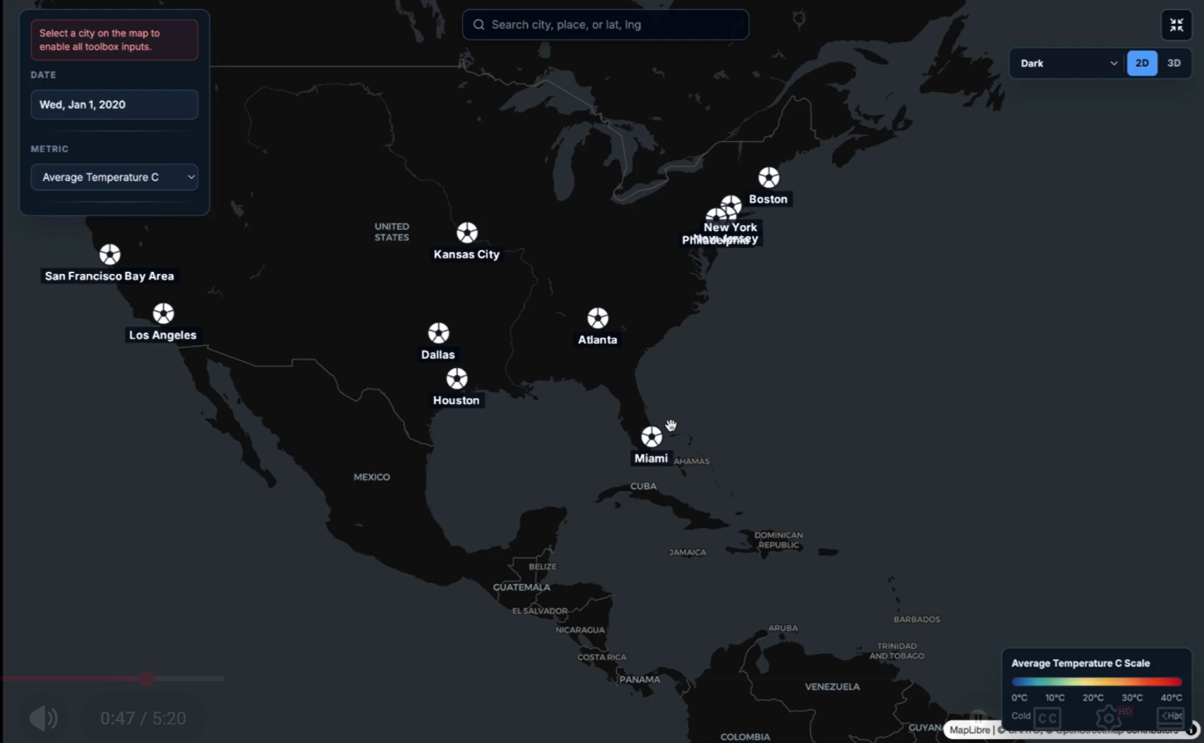
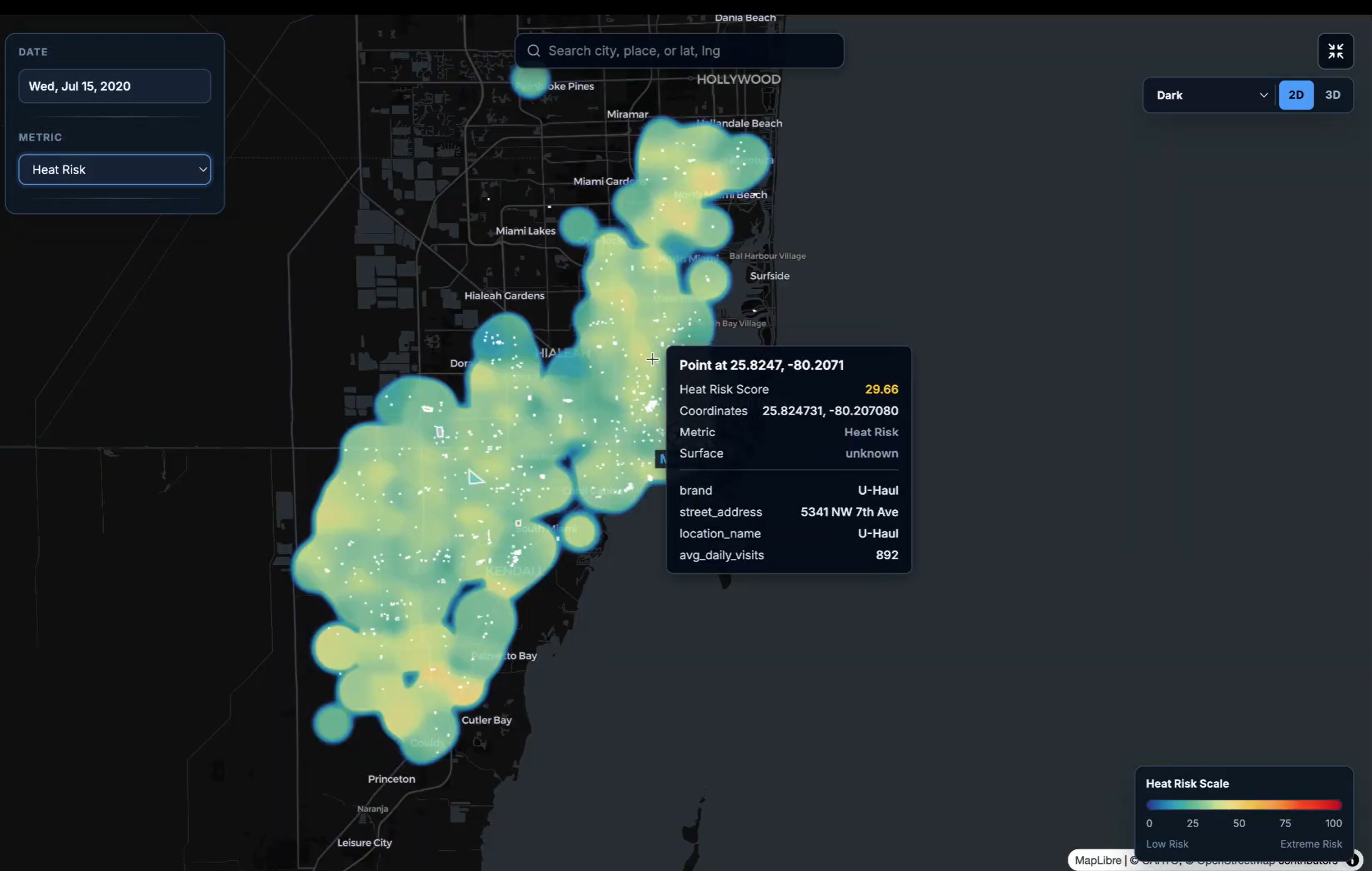
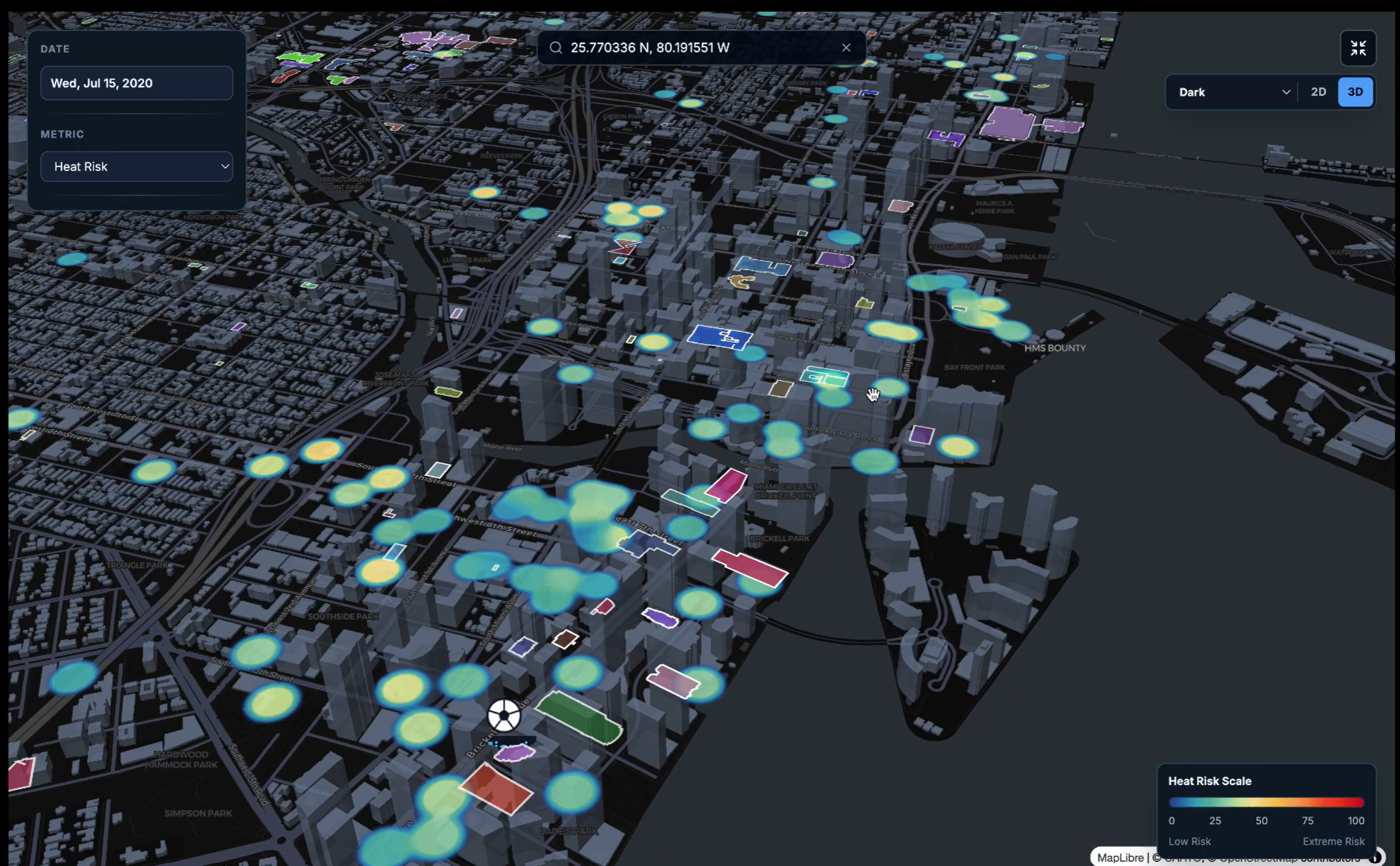
In Explore mode, planners can select host cities and inspect interpolated heat-map layers for metrics such as visitor density and heat risk. They can also view key points of interest. This creates an interactive view of baseline conditions and provides context for later intervention scenarios.

Simulation Mode

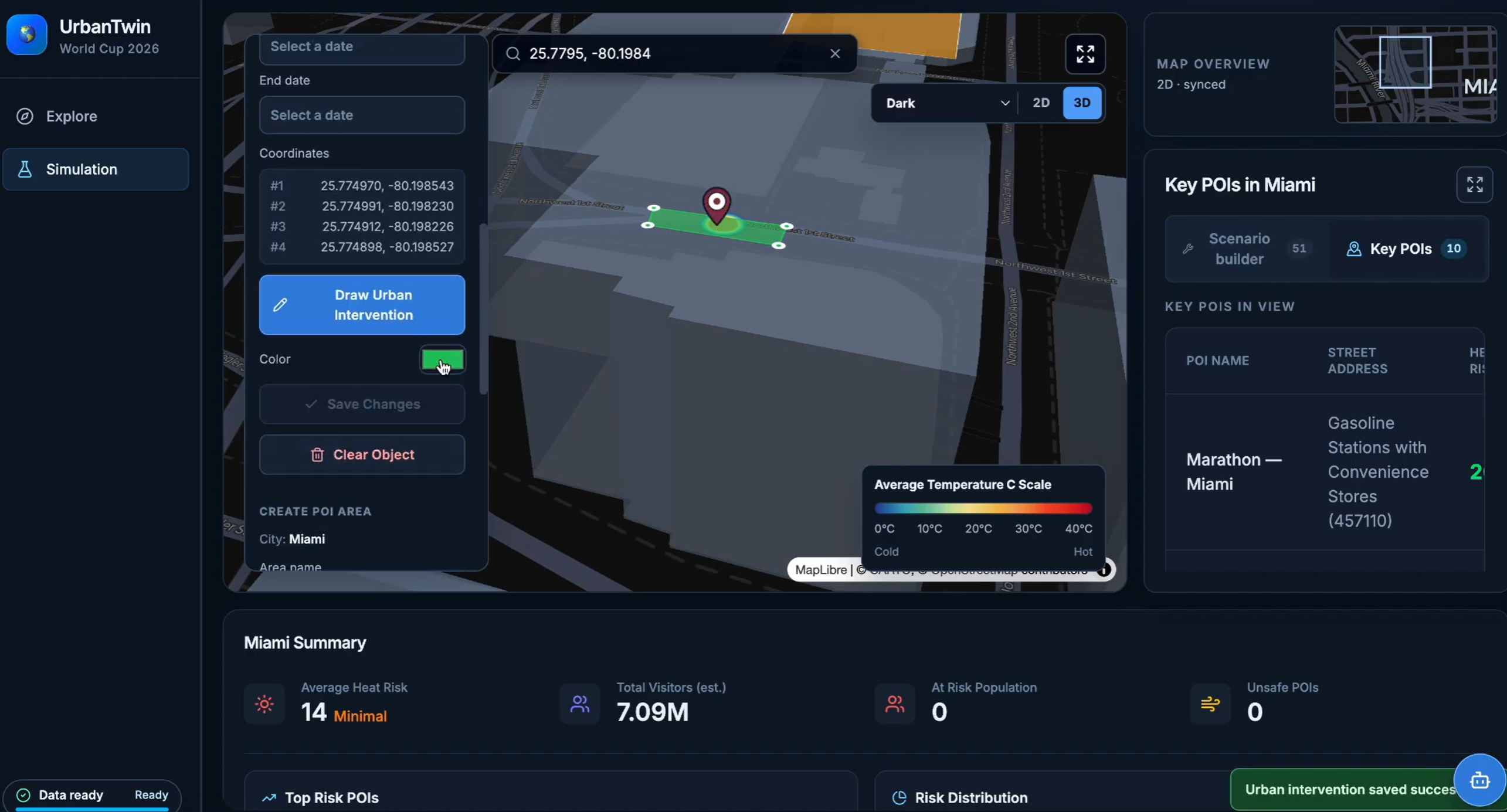
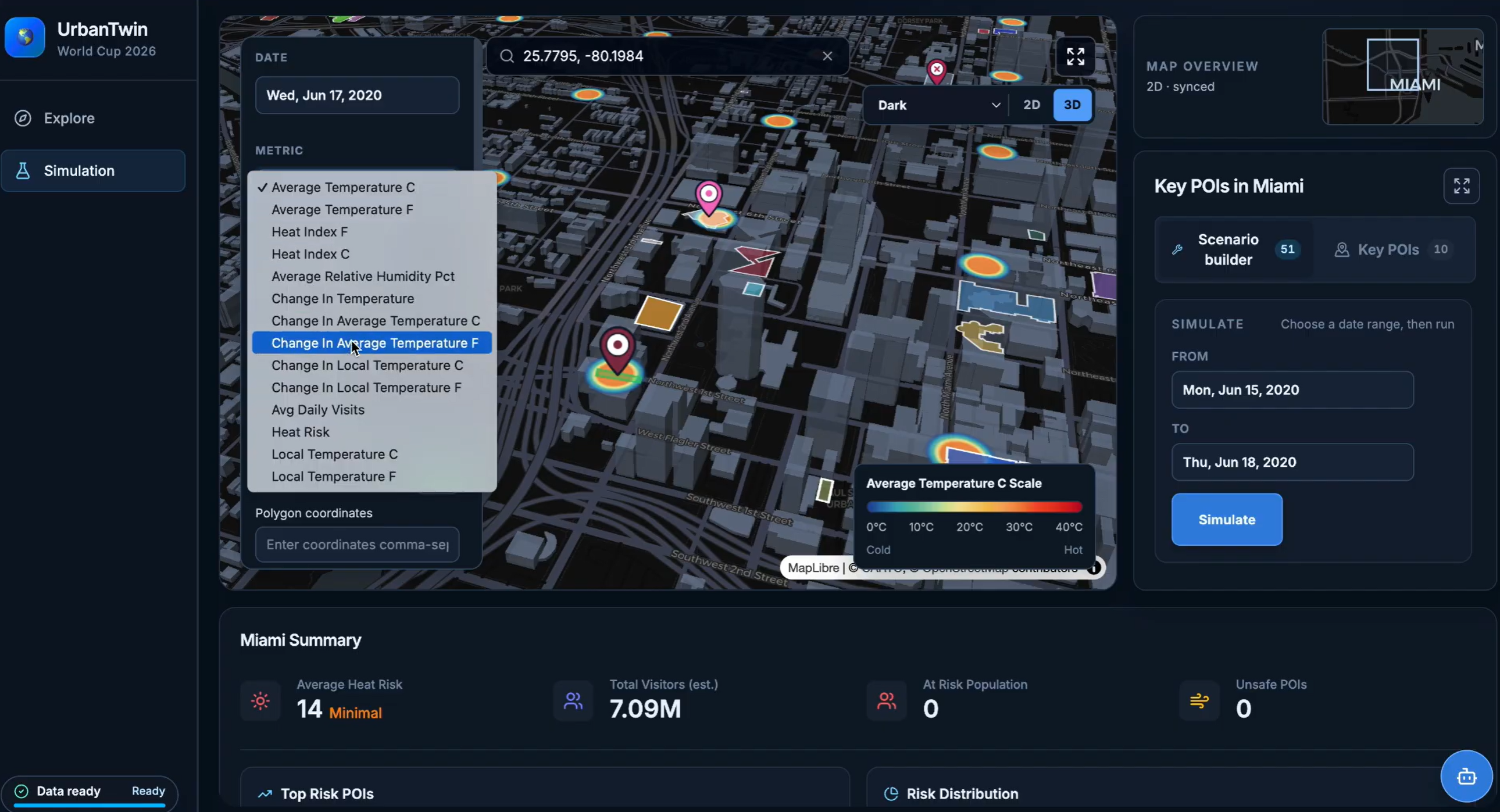
In Simulation mode, planners can explore city-level heat risk and key points of interest, select a time period, draw target areas, and place potential interventions directly on the map.

The platform models four heat-mitigation approaches:

Vegetation, such as street trees, parks, green roofs, and rain gardens.
High-albedo surfaces, such as cool roofs and reflective pavement.
Shade structures, such as canopies, awnings, shade sails, and bus shelters.
Evaporative cooling, such as fountains, splash pads, and misting systems.

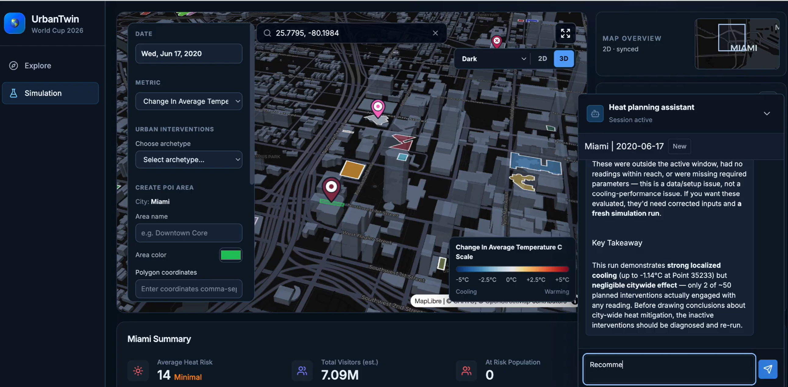
Planners can drag and drop interventions onto target locations, define their area of impact, and set active dates. The platform applies weather-aware cooling models and displays resulting changes through an updated heat map and timeline. This allows planners to compare scenarios, identify high-risk areas, and prioritize practical investments that improve heat safety during future mega-events.

Together, Explore and Simulation modes allow planners to select a host city, interact with its metrics, test interventions, and understand how those interventions work within the city’s environmental conditions. The goal is to help officials identify priority areas, make data-informed investments, and prepare safer, more resilient host cities before visitors arrive.

How We Built It

Frontend

We built the frontend with React and TypeScript, using Vite for development and bundling and Tailwind CSS for styling. Explore and Simulation share a map-centered interface with city selection, metric controls, date selection, points of interest, and summary statistics.

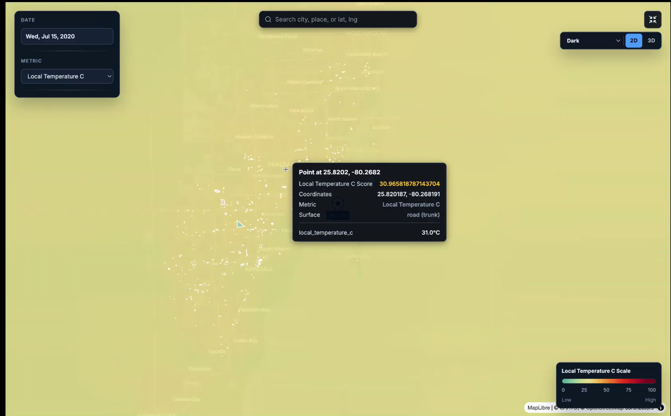
MapLibre GL renders the basemap, while deck.gl supplies GPU-accelerated heat-map, polygon, point, and icon layers. The map cameras stay synchronized as users pan and zoom. The heat-map layer blends nearby values using weighted-mean aggregation, with fixed color domains for each metric so the scale stays consistent across dates. A separate interactive point layer supports tooltips that show the underlying point values. Temperature-change views use blue for cooling and red for warming.

Custom React hooks organize polygon drawing, intervention placement, map-layer construction, and timeline playback. Planners can place interventions, define their footprints and active dates, and send a scenario to the FastAPI backend. The returned results are grouped by date and played back on the map, making changes over time easier to inspect. TypeScript interfaces define the data exchanged between the interface and API, while memoized layers and cancellation of outdated requests help keep interactions responsive.

Backend

We use a FastAPI and SQLAlchemy Python-based backend organized around routers, services, and repositories. Business logic lives in service files, database querying lives in repository files, and API endpoints live in router files. The platform is backed by a live Neon-hosted PostgreSQL database.

To keep the platform responsive with large datasets and to support future multi-user scale, we combine Redis caching and preloading with Celery background workers for asynchronous processing and concurrent weather-data retrieval. This reduces repeated API calls and helps keep maps and simulations responsive.

Machine Learning and Statistics

The current prototype combines geospatial statistics, stored visitor and heat-risk data, and weather-aware mathematical simulation. The repository implements Ordinary Kriging through PyKrige for estimating available metrics at unsampled grid-cell centroids. It preserves existing values and calculates interpolation variance, which is converted into a relative confidence score within each interpolation run. This score describes relative interpolation uncertainty; it is not a calibrated probability of predictive accuracy.

The data layer includes daily weather records, urban heat-island measurements, store-visit records, and point-of-interest geometry. The repository also defines spending datasets for additional economic context and includes a National Weather Service integration. Coordinates, city or market identifiers, and dates connect environmental conditions with locations and visitor activity. The visitor API serves stored average daily visits and heat-risk scores and calculates summaries such as total visits, average risk scores, and visit-weighted heat-index categories.

These data support baseline map exploration, while the intervention models estimate temperature changes under a selected scenario. Backend spatial interpolation and frontend heat-map smoothing serve different purposes: kriging estimates missing spatial values, and deck.gl blends values for display.

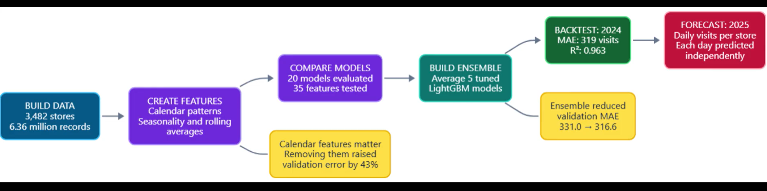
The repository includes automated tests for visitor aggregation, heat-risk classification, missing-data handling, intervention parameter validation, and geometry conversion, alongside sample simulation scripts. These check software behavior. The published code does not include a reproducible supervised-learning training pipeline, the derivation of the stored heat-risk scores, or held-out accuracy results. Field calibration and comparison with independent observations remain necessary before claiming validated predictive performance.

Rice-To-Meet-You simulates how urban cooling interventions change pedestrian-level temperature across a date-indexed heat map. A planner draws or places an intervention, selects when it is active, and the model recalculates map points inside its footprint, or within its cooling radius for water-based interventions.

Ordinary Kriging Interpolation

To display continuous metric values across city grid cells, we use Ordinary Kriging with a linear variogram. Known metric readings estimate values at unsampled grid-cell centroids.

The predicted value at an unsampled location is:

$$ \hat{z}(s_0) = \sum_{i=1}^{n} \lambda_i z(s_i) $$

subject to the unbiasedness constraint:

$$ \sum_{i=1}^{n} \lambda_i = 1 $$

The kriging weights and Lagrange multiplier are calculated by solving, for each known point $s_i$:

$$ \sum_{j=1}^{n} \lambda_j\,\gamma(s_i-s_j) + \mu = \gamma(s_i-s_0), \qquad i = 1, \ldots, n $$

The platform uses a linear variogram:

$$ \gamma(h) = \text{slope} \cdot h + \text{nugget} $$

Where:

$\hat{z}(s_0)$ is the predicted metric value at target centroid $s_0$.
$z(s_i)$ is the observed value at known point $i$.
$\lambda_i$ is the weight assigned to known point $i$.
$\gamma(h)$ is semivariance at distance $h$.
$\mu$ is a Lagrange multiplier enforcing unbiased interpolation.

Known grid cells keep their exact observed values; Ordinary Kriging predicts only unsampled grid-cell centroids, creating the continuous heat-map layer.

Weather Conditions

The model calculates saturation vapor pressure:

$$ e_s(T) = 0.6108 \times e^{\frac{17.27 \times T}{T + 237.3}} $$

It then calculates vapor-pressure deficit:

$$ VPD = e_s(T) \times \left(1 - \frac{RH}{100}\right) $$

Where T is temperature in degrees Celsius and RH is relative humidity percentage.

Vegetation Cooling

Vegetation combines cooling from shade and evapotranspiration.

$$ \Delta T_{\max} = 5 \times f_{VPD} \times f_{solar} \times f_{wind} $$

$$ f_{VPD} = \min\left(\frac{VPD}{4.5}, 1\right) $$

The leaf-area effect uses a saturating Beer–Lambert relationship:

$$ f_{LAI} = 1 - e^{-0.5 \times LAI} $$

$$ I_{vegetation} = 0.4 \times (C \times f_{LAI} \times W)

0.6 \times (C \times K \times f_{LAI} \times (0.8 + 0.2 \times W)) $$

$$ \Delta T = \Delta T_{\max} \times I_{vegetation} $$

Where C is vegetation coverage, K is canopy fraction, LAI is leaf-area index, and W is irrigation or water availability.

High-Albedo Surface Cooling

Reflective surfaces reduce absorbed solar energy.

$$ \Delta T_{\max} = 4 \times f_{thermal} \times f_{solar} $$

$$ f_{thermal} = \mathrm{clamp}\left(\frac{T - 20}{38 - 20}, 0, 1\right) $$

$$ I_{albedo} = \min\left(\frac{\Delta \alpha}{0.7}, 1\right) \times A $$

Where Δα is albedo improvement and A is treated-area coverage.

Shade-Structure Cooling

Shade structures reduce direct solar exposure.

$$ \Delta T_{\max} = 5 \times f_{thermal} \times f_{solar} \times 0.85 $$

$$ I_{shade} = O \times A $$

Where O is shade opacity and A is shaded-footprint coverage.

Evaporative Cooling

Water-based interventions are strongest in hot, dry conditions and diminish with distance.

$$ \Delta T_{\max} = 8 \times f_{VPD} \times f_{wind} $$

$$ P = \left(\frac{Q}{60}\right) \times 2.45 \times 10^6 $$

$$ I_{source} = \min\left(\frac{P}{50,000}, 1\right) $$

$$ f_{distance} = \max\left(1 - \frac{r}{R}, 0\right) $$

$$ \Delta T = \Delta T_{\max} \times I_{source} \times D \times f_{distance} $$

Where Q is evaporation rate in liters per minute, r is distance from the cooling source, R is cooling radius, and D is active fraction or duty cycle.

Diminishing-Return Simulation

When multiple interventions overlap, the simulation prevents unrealistic stacking of cooling benefits. It combines intervention effects against the same local cooling ceiling:

$$ Impact = 1 - \prod_i \left[ 1 - \mathrm{clamp}\left(\frac{c_i \times F}{C}, 0, 1\right) \right] $$

$$ \Delta T_{combined} = C \times Impact $$

Where cᵢ is an individual intervention’s cooling contribution, C is the local cooling ceiling, and F is a contextual interaction factor.

For example, vegetation and water-based cooling can reinforce one another, while vegetation and shade structures can have partially redundant benefits because both reduce solar exposure.

Challenges

This project was ambitious. Four developers contributed around internship schedules and across Houston, Pittsburgh, and Vietnam. Below are the principal challenges and our responses.

Time coordination and meetings: We originally planned at least three meetings per week. As internships intensified and team members returned to university, availability decreased and time conflicts increased. We shifted to asynchronous communication, agile sprints, a clear task list, shared weekly meeting notes, and frequent progress reports to keep the team on track.
Different technical backgrounds: Team members had different areas of specialization, which sometimes made feature handoffs difficult. We addressed this by teaching the basics of the relevant technology and preparing short, non-technical slide presentations before major implementation discussions.
Distributed development: Parallel feature work sometimes created over- or under-engineered implementations and merge conflicts caused by overlapping changes or outdated assumptions. We improved this process through stricter testing, including unit tests, property-based tests, and GitHub integration tests, before merging work into the main codebase.

Accomplishments That We’re Proud Of

Built an end-to-end interactive planning prototype, combining a React map interface with a FastAPI, PostgreSQL, and Redis-backed data platform that is hosted and deployed live.
Turned abstract heat-risk data into an accessible, grid-level visualization that helps planners explore risk at specific locations and points of interest.
Created a simulation workspace where users can draw intervention areas and test vegetation, reflective surfaces, shade structures, and evaporative-cooling strategies modeled after environmental research and formulas.
Made simulations weather-aware by accounting for temperature, humidity, solar exposure, wind, coverage, and intervention intensity.
Designed for real-world scale through live database support, cached data, concurrent weather retrieval, and asynchronous background processing.
Delivered a cohesive tool despite a distributed team working across three locations and demanding internship schedules.

What We Learned

Technical Challenges

Although AI quickly reduced many technical challenges, we soon realized it provided diminishing returns as the codebase grew. As our code increased in size, complexity, and features, we quickly realized that sometimes, it became our bottleneck.
For the backend, the biggest challenge was making code that was clean, well-documented, and scalable. Since our database was deployed on NeonDB, an online PostgreSQL provider, every time we called our API and routes, we were billed a small amount. So we had to optimize our routes and data calls and implement a Grafana dashboard to monitor usage and cost.

Team Challenges

The hardest part of the hackathon was not only programming or feature development. It was conveying information clearly, managing a four-person team across time zones, and keeping everyone aligned on the same goal.
A huge challenge was working around technology constraints: database storage constraints and data-transfer/loading-speed constraints.
Data context matters as much as data volume: Connecting weather, visitor activity, and urban heat measurements requires consistent locations, dates, units, and geographic scales. Store visits provide a useful indicator of activity, but they do not directly measure simultaneous crowd density or unique people. Missing observations also need to remain distinguishable from a true zero.
Useful simulations need explicit assumptions: Cooling depends on local weather, intervention coverage, operating dates, and interactions between interventions. Modeling diminishing returns helps prevent overlapping interventions from producing unrealistic benefits. These assumptions make scenario comparisons more interpretable and show where future field measurements would improve calibration.
Visualization is part of the analysis: A smooth heat map can make sparse data appear more precise than they are. Consistent color scales, access to underlying point values, and clear separation between baseline conditions and simulated temperature changes help planners interpret the results responsibly.