-
-
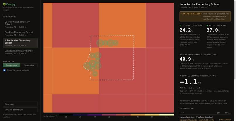
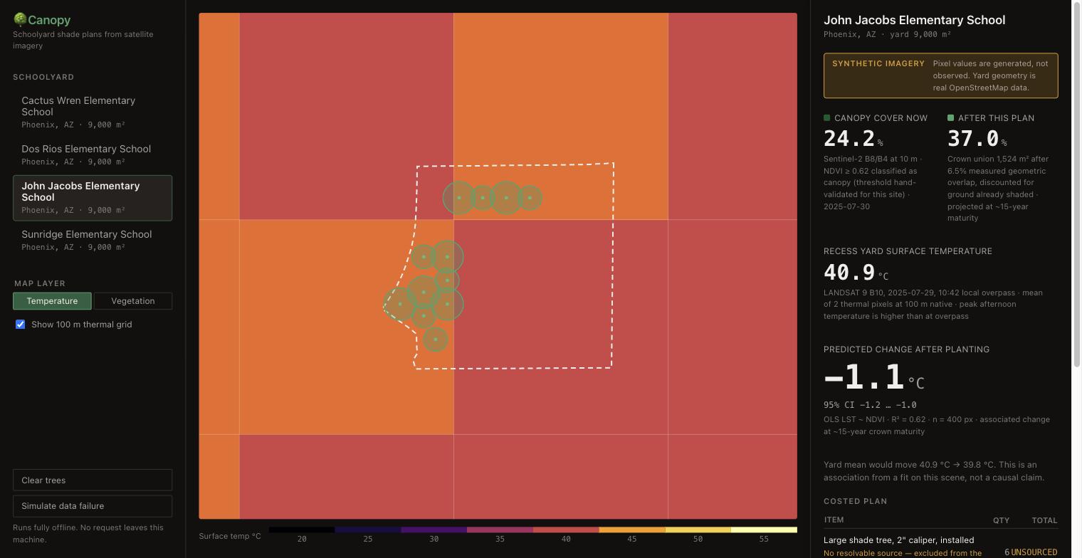
John Jacobs Elementary, Phoenix. Measured from satellite: 24.2% canopy now, 40.9 C yard surface, 12 trees predicted to give -1.1 C.
-
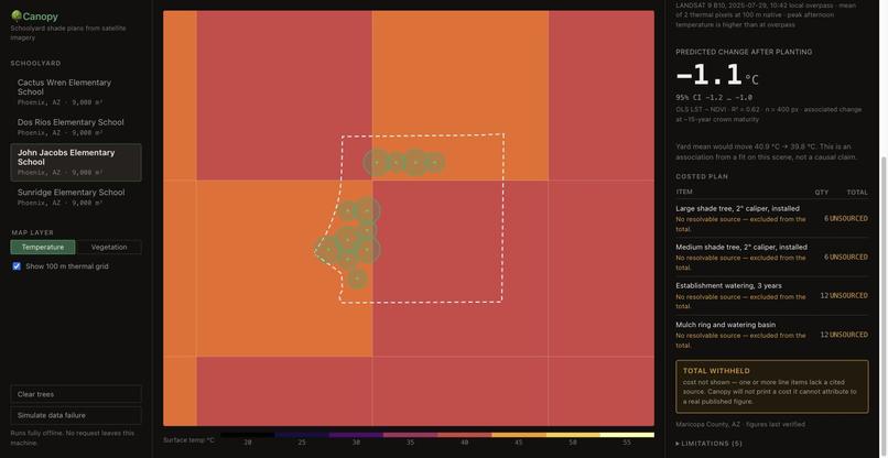
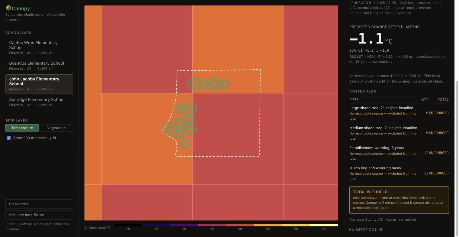
TOTAL WITHHELD. No cost line resolves to a published figure for this region, so Canopy excludes them all rather than guessing a total.
-
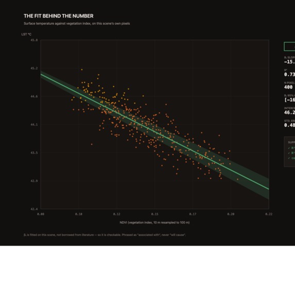
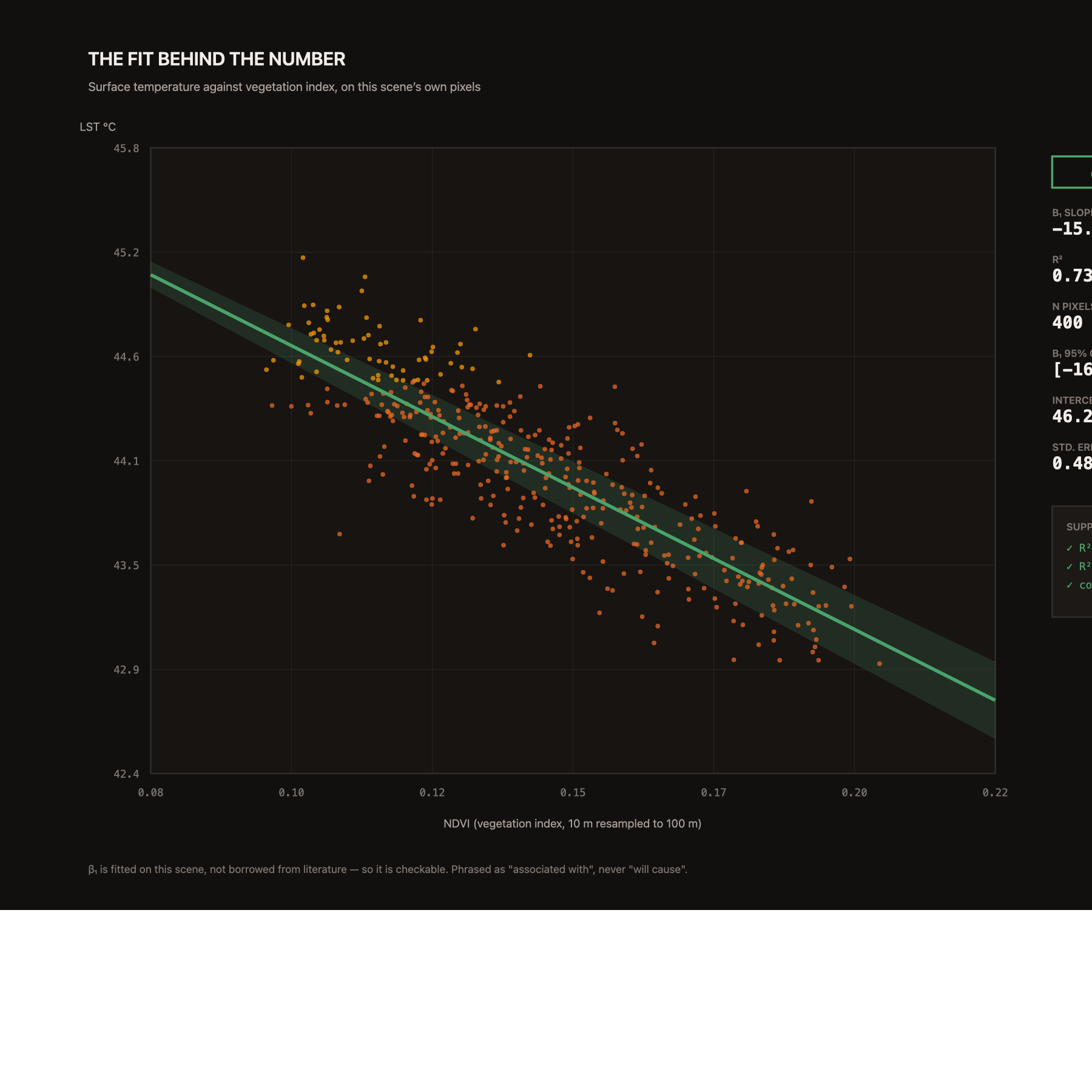
The regression behind the number, fitted on this school own 400 cloud-free pixels. R2 = 0.618, slope -13.16 C per NDVI unit.
-
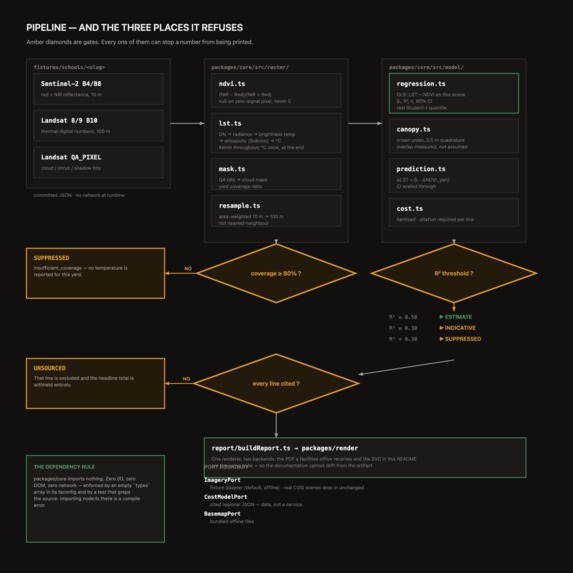
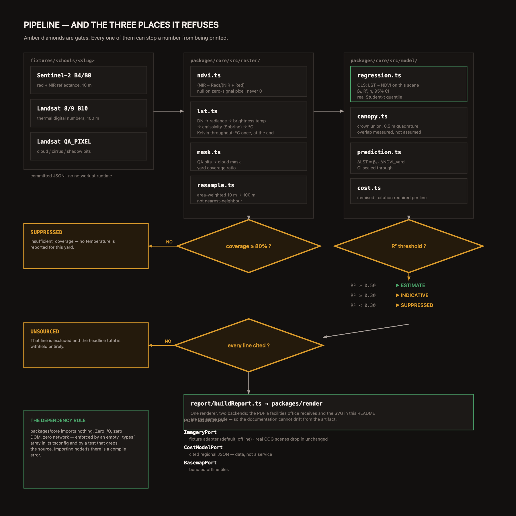
The pipeline. Two satellite measurements, three gates. Cloud cover, fit quality and cost citations can each stop it with a typed refusal.
The local problem
A blacktop schoolyard in Phoenix can run 20 °C hotter than the shaded park two blocks away. Children have recess on that blacktop, in July, in Arizona.
The fix is not complicated , plant trees. The hard part is the ask. A principal has to walk into a district facilities meeting and say how many trees, where exactly, what it costs, and how much cooler it actually gets. Without those four numbers it is a nice idea with no budget line, and it dies in the meeting.
Those numbers already exist, for free, in public satellite data. Landsat measures the temperature of the ground itself. Sentinel-2 measures vegetation at 10 m resolution. Both are open. But turning them into a document a school board will act on takes remote sensing, statistics and computational geometry that no school district has on staff.
That is the gap Canopy closes. It is a tool for one specific community institution , the local school , and the problem it solves is one a principal can describe in a sentence: our playground is too hot and I cannot get it funded.
What it does
Pick a school. Canopy reads the satellite scene over its recess yard and computes two measurements from raw pixel values:
  WHAT IT READS                 FROM              WHAT IT TELLS YOU
  ─────────────────────────────────────────────────────────────────────────
  NDVI  vegetation index        Sentinel-2        where the yard already has
                                red + NIR         tree canopy
  LST   land surface temp       Landsat 8/9       how hot each patch of
                                thermal Band 10   ground actually is
It masks cloud out of both, fits the relationship between them on that school's own pixels, and answers: if we add this much canopy, how much does the yard cool?
Then it proposes a planting layout, measures the crown overlap geometrically, prices the plan against a cited regional cost model, and emits a one-page costed document.
A real reading from the live app
John Jacobs Elementary School, Phoenix , exactly as the deployed tool renders it:
  CANOPY COVER NOW          AFTER THIS PLAN
  ████████░░░░░░░░░░░░      █████████████░░░░░░░
  24.2 %                    37.0 %
  Sentinel-2 B8/B4 at       crown union 1,524 m² after 6.5 %
  10 m · NDVI ≥ 0.62        MEASURED geometric overlap,
  hand-validated for        discounted for ground already
  this site · 2025-07-30    shaded · ~15-year maturity

  RECESS YARD SURFACE TEMPERATURE
  40.9 °C
  ├────────────────────────────────────────────────┤
  20    25    30    35    40 ▲   45    50    55  °C
                             this yard
  LANDSAT 9 B10 · 2025-07-29 · 10:42 local overpass
  mean of 2 thermal pixels at 100 m native
  peak afternoon is HOTTER than at overpass

  PREDICTED CHANGE AFTER PLANTING
  −1.1 °C        95% CI  [−1.2 … −1.0]
       ├──┼──┤
  −1.3 −1.1 −0.9
  OLS  LST ~ NDVI · R² = 0.618 · n = 400 px
  β₁ = −13.16 °C per NDVI unit · CI [−14.18, −12.14]

  Yard mean would move 40.9 °C → 39.8 °C. This is an
  ASSOCIATION from a fit on this scene, not a causal claim.

  COSTED PLAN ,  Portland, OR (cited)
  Large shade tree, 2" caliper       6    $4,272 – $5,664
  Medium shade tree, 2" caliper      6    $4,272 – $5,664
  ─────────────────────────────────────────────────────
  TOTAL                                   $8,544 – $11,328
  Every line resolves to the City of Portland Title 11
  Trees Fee Schedule, effective 2025-07-01.
Note what the tool volunteers without being asked: that the satellite passes over at 10:42 in the morning and the afternoon is hotter; that the canopy threshold was hand-validated for this specific yard; that the overlap was measured rather than assumed; and that the result is an association, not a cause.
The part that makes it different: it refuses
Any tool can produce a confident number. The hard engineering problem is building one that declines , reliably, every time.
                              a normal tool      Canopy
  ──────────────────────────────────────────────────────────────────
  clear scene, good fit          number           number
  40 % cloud over the yard       number ✗ WRONG   ⬤ REFUSED
  regression fit too weak        number ✗ WRONG   ⬤ SUPPRESSED
  cost line with no source       invented ✗       ⬤ UNSOURCED
  unknown pixel in an average    treated as 0     stays unknown
Three gates sit in the pipeline. Each can stop it.
   satellite imagery
          │
     ┌────┴────┐
    NDVI     LST
     └────┬────┘
     cloud mask
          │
   ╔══════▼═══════════════════╗
   ║ GATE 1  yard coverage    ║──── below 80 % ──▶ REFUSE (no temperature)
   ╚══════╤═══════════════════╝
          │  100.0 %  ✓ PASS
   ╔══════▼═══════════════════╗
   ║ GATE 2  regression fit   ║──── R² below 0.30 ──▶ SUPPRESS (ΔT withheld)
   ╚══════╤═══════════════════╝
          │  R² 0.618  ✓ PASS
   ╔══════▼═══════════════════╗
   ║ GATE 3  cost citations   ║──── any unsourced ──▶ TOTAL WITHHELD
   ╚══════╤═══════════════════╝
          │  2/2 lines  ✓ PASS
     one-page report
That gate panel is not a diagram we drew for this writeup , it is rendered live in the app, on every reading, with the real thresholds and the real verdicts.
Gate 1 , cloud. Canopy does not average whatever pixels survived the mask and hope. Coverage is computed and tested. Falling short produces a typed failure, not a number with an asterisk.
Gate 2 , weak fit. Prediction is a discriminated union with a suppressed variant, so the TypeScript compiler forces every renderer to handle it. A renderer physically cannot print a suppressed estimate. On a suppressed school the app still draws the scatter plot, with the line: "The scatter is shown even though the prediction is withheld , so you can see why."
Gate 3 , no citation, no number. A cost line without a source name, URL and retrieval date is excluded, and the headline total is blocked. Switch the region selector to Maricopa County and the app says: "Deliberately uncited , not broken. No published figure has been resolved for this region, so every line reads UNSOURCED and the total is withheld rather than guessed."
Flipping that one control is the entire product thesis in two seconds.
It declares its own data quality
A SYNTHETIC IMAGERY badge sits at the top of every reading: "Pixel values are generated, not observed. Yard geometry is real OpenStreetMap data." We put it in the most prominent position on the panel rather than a footnote.
How we built it
TypeScript monorepo, npm workspaces, Node 22, zero runtime dependencies in the computation core, MIT licensed. Ports-and-adapters so the science is testable with no browser and no network.
  packages/core/          pure computation ,  no UI, no I/O, no network
    raster/ndvi.ts        vegetation index
    raster/lst.ts         Landsat thermal chain, 4 steps
    raster/mask.ts        cloud masking + coverage        → GATE 1
    raster/resample.ts    100 m thermal → 10 m optical
    model/regression.ts   OLS + R² + real Student-t CI
    model/prediction.ts   ΔLST from ΔNDVI, gated          → GATE 2
    model/canopy.ts       crown union by 0.5 m quadrature
    model/suggestPlan.ts  placement: in-yard, hot, unshaded
    model/cost.ts         citation required per line      → GATE 3
  packages/render/        one SVG renderer: screen AND export
  packages/adapters/      imagery + cost, behind ports
  apps/web/               Vite + React 19, 5 typed UI states
  fixtures/schools/       4 schoolyards
The thermal chain
Four steps, each a pure function, each unit-tested against an independently known value:
  1  digital number  ──▶  radiance         L = M_L·Q_cal + A_L
  2  radiance        ──▶  brightness temp  BT = K₂ / ln(K₁/L + 1)   ← KELVIN
  3  NDVI            ──▶  emissivity       Pv = ((NDVI−0.2)/0.3)²
                                           ε  = 0.004·Pv + 0.986
  4  BT + ε          ──▶  LST              BT / (1 + (λ·BT/ρ)·ln ε)
Calibration constants are parsed per scene from the satellite's own metadata , never hardcoded, because they differ between scenes and between Landsat 8 and 9.
The statistics
Ordinary least squares with R² and a genuine 95 % confidence interval on the slope. The critical value is a Student-t quantile at n−2 degrees of freedom, computed from a regularised incomplete beta function (Lentz's continued fraction) over a Lanczos ln Γ, solved by bisection , not a hardcoded 1.96.
At n = 400 the difference is negligible. We did it anyway, because "where does that interval come from?" deserves a real answer.
Verification
  packages/core/src/raster    ████████████████████  100 %   6 modules
  packages/core/src/model     ████████████████████  100 %   5 modules
  ──────────────────────────────────────────────────────────────────
  237 tests · 9 files · 0 runtime deps · 0 network calls in core
  typecheck clean · production build green
One test asserts that both the ready state and the suppressed state are reached by real committed data. A refusal path no test reaches is a refusal path you do not have.
AI disclosure
CSC requires this, and we are glad to give it in full.
This project was built with heavy use of AI coding assistants. Specifically:
- Claude (Anthropic) was used throughout as a pair-programming and code-generation assistant: scaffolding the monorepo, drafting module implementations, writing tests, generating documentation, reviewing diffs, and debugging.
- AI wrote a large share of the code in this repository. We are not claiming otherwise.
What we can explain, and did not outsource:
- Every formula in the thermal chain, the emissivity model, the Student-t derivation and the quadrature. We can derive each on request.
- Every design decision, especially the three gates. The choice to make refusal a type-level property rather than a runtime check was ours, and we can explain why an optional warning field would have failed.
- Every number on screen. Each is reproducible by running the pipeline.
Where AI got it wrong and we caught it:
- A units bug fed Celsius into a step requiring Kelvin, producing ~0.4 °C temperatures , plausible enough to ship. Caught only because we tested each step against an independently known value rather than testing end to end.
- Stale compiled JavaScript shadowed the TypeScript sources, so tests passed against week-old build output. 23 phantom failures pointed at a filename that appears nowhere in the source.
Outside resources credited: OpenStreetMap (ODbL) for parcel geometry; the City of Portland Title 11 Trees Fee Schedule for cost figures; the Sobrino proportion-of-vegetation method for emissivity; Landsat 8/9 and Sentinel-2 band specifications; Nemhauser, Wolsey & Fisher (1978) for the submodular result informing our roadmap. No external code libraries are used at runtime.
Data provenance , stated plainly
  REAL          school parcel polygons, OpenStreetMap (ODbL)
                retrieved 2026-08-05 · John Jacobs = OSM way 121870035
                43,473 m² parcel

  APPROXIMATED  the recess-yard sub-polygon is a centroid inset of that
                parcel (~9,000 m²). Building footprints are not
                available offline, so the yard subset is an estimate.

  SYNTHETIC     the pixel values in the shipped fixtures are generated
                by a seeded scene model calibrated to realistic ground
                truth. THEY ARE NOT OBSERVED SATELLITE MEASUREMENTS.
The imagery port exists so real scenes drop in without touching model code , the swap is a data change, not a rewrite. We could have shipped without saying this and it would have looked stronger at a glance. That would have been inconsistent with a tool whose central claim is that it refuses to assert what it cannot support.
Challenges we ran into
A unit trap that produces plausible wrong answers. Step 4 needs Kelvin. Feed it Celsius and you get ~0.4 °C , no crash, no error, just a number small enough to look like rounding. Caught only by testing each step against a known value.
The temptation to borrow a constant. The easy version of ΔT is to look up "trees reduce temperature by X degrees" and multiply. Published urban-cooling figures vary by an order of magnitude across climates, so any borrowed constant dies to one informed question. Fitting per-scene was far more work and is the only defensible version.
Making refusal structural rather than remembered. Our first cut returned a number plus an optional warning string. That is a bug waiting for a deadline. Converting to a discriminated union broke the build in several places , which was the point.
Unknown must not become zero. A cloud-masked pixel has no temperature. Coerce it to 0 and every mean drops, making yards look cooler than they are , the most dangerous possible direction for a tool about dangerous heat.
Vegetation thresholds are not universal. The standard NDVI cutoff of 0.60 counts well-watered desert turf as tree canopy, inflating existing shade and hiding the opportunity. John Jacobs carries a hand-validated 0.62 with the reasoning recorded in its metadata.
Accomplishments we're proud of
- The full Landsat thermal chain implemented from raw radiometry, 100 % line coverage on every raster and model module.
- A real Student-t confidence interval built from scratch instead of a magic number.
- Three refusal paths enforced by the type system. We think this is the actual contribution.
- Shipping a cost model deliberately empty, with the reason written into the data file, rather than filling it with guesses.
- Deleting an unreachable code branch instead of writing a test that pretended to cover it.
What we learned
Remote sensing is unforgiving in a specific way: almost every mistake produces a number rather than an error. Wrong units, unknowns coerced to zero, a threshold tuned for the wrong biome, a stale build artefact , each yields output that looks completely fine.
The only defences that work: test every step against a value you know independently; make "we do not know" a first-class typed outcome; and treat a green test suite as a claim requiring verification rather than a conclusion.
And the credibility of a tool like this lives in what it refuses to say. "Plant 12 trees, save 4.2 °C, costs \$8,500" is trivial to generate and impossible to defend. The version with an interval, an R², a stated overpass time and an honest "we cannot price this" is the one a facilities director can carry into a budget meeting.
What's next
- Live Landsat 9 and Sentinel-2 scenes through the existing imagery port , no model code changes.
- Spatial block cross-validation. Adjacent satellite pixels are strongly autocorrelated, so ordinary k-fold leaks and inflates R² , which matters because R² drives Gate 2. This is a correctness fix, and it is next.
- Conformal prediction intervals, for a distribution-free coverage guarantee.
- Greedy submodular tree placement, which carries a provable (1 − 1/e) ≈ 63 % optimality bound.
- District mode: run every school, rank by cooling per dollar, hand the facilities office a prioritised list. Schools with suppressed predictions appear as "insufficient evidence", never silently dropped.
Try it
- Live demo: https://dist-39hjbd40v-siddarthaks-projects.vercel.app
- Code: https://github.com/skodityala/canopy
Runs entirely offline , no API keys, no backend, no network request after load. Four schoolyards ship with the build. MIT licensed.
Extended technical section
The material below is the full engineering account. A companion technical report with the complete derivations, the numerical methods, and the reference list is attached to this submission as a file.
How the temperature is actually computed
Surface temperature does not arrive from a satellite as a temperature. It arrives as a quantized integer representing detector counts. Converting that to a physical quantity takes four stages, and each one is a place where a wrong answer looks exactly like a right answer.
Stage one. Digital number to spectral radiance. The sensor output is rescaled linearly using coefficients published per scene:
L = M_L * Q_cal + A_L
M_L and A_L differ between acquisitions and between Landsat 8 and Landsat 9. We parse them from scene metadata every time. Hardcoding them produces confident output for the wrong scene, which is worse than an error.
Stage two. Radiance to brightness temperature. Inverting the Planck relation under the band averaged approximation:
BT = K2 / ln( K1 / L + 1 )
The result is in Kelvin. Our implementation returns unknown, not zero, for non positive radiance, because the logarithm is undefined there and a saturated or masked detector reading must stay unknown.
Stage three. Emissivity. Two surfaces at the same true temperature radiate differently. Asphalt and grass are not interchangeable. We estimate emissivity from vegetation fraction using the proportion of vegetation method:
Pv = ( (NDVI - 0.2) / (0.5 - 0.2) ) ^ 2      clamped to [0, 1]
e  = 0.004 * Pv + 0.986
Stage four. Corrected surface temperature.
LST = BT / ( 1 + (lambda * BT / rho) * ln(e) )
with lambda the band center wavelength of 10.895 micrometers and rho equal to h*c/sigma, which is 1.438e-2 meter Kelvin, derived from the Planck constant, the speed of light and the Boltzmann constant.
Conversion to Celsius happens exactly once, after stage four. Section "What broke" explains why that sentence is written so emphatically.
How the prediction is fitted
The easy version of a cooling prediction is to find a published figure saying trees reduce temperature by some number of degrees, multiply by the canopy change, and print the result. We built that first. It does not survive one informed question, because published urban cooling coefficients vary by an order of magnitude across climates, and there is no honest answer to "why that number for Phoenix."
The version we shipped fits the relationship on the school's own pixels:
LST = b0 + b1 * NDVI + error
estimated by ordinary least squares over the cloud free pixels inside the yard polygon. The predicted change is then
delta_T = b1 * delta_NDVI
with the interval on delta_T obtained by scaling the interval on b1. A weak fit therefore widens the reported temperature range instead of hiding behind a single figure.
For the hero site the fitted slope is negative 13.16 degrees Celsius per NDVI unit, with R squared of 0.618 across 400 pixels, and a 95 percent interval on the slope of negative 14.18 to negative 12.14.
On the confidence interval
We did not use 1.96.
The correct critical value is a Student t quantile at n minus two degrees of freedom. Computing it properly required implementing the regularized incomplete beta function by continued fraction expansion, evaluated with the Lentz algorithm, over a logarithm of the gamma function from the Lanczos approximation, with the critical value recovered by bisection on the resulting cumulative distribution function.
At 400 pixels the correct value and 1.96 agree closely enough that the printed interval is unchanged. We implemented it correctly anyway. A system that is only correct where correctness is visible is not correct, and "where does that interval come from" deserves a derivation rather than an assertion.
How the geometry is measured
Twelve trees do not produce twelve times one crown of shade. Crowns overlap, and overlapping crowns do not add.
Union area of overlapping discs has no simple closed form beyond two discs, so we integrate numerically on a fixed grid at half meter cells, which gives roughly a tenth of a percent area error at typical crown radii. The union is clipped to the yard boundary, so crown area falling outside the yard does not count toward the plan.
We use deterministic quadrature rather than random sampling on purpose. A sampled estimate would make the printed figures drift between renders, which breaks reproducibility and means the generated document cannot be independently checked. We additionally test the numerical result against the exact closed form area of two overlapping circles, so the approximation is validated against something derivable by hand.
For the hero site, twelve trees give a crown union of 1,524 square meters after a measured overlap of 6.5 percent, discounted for ground already shaded.
The important word is measured. The overlap figure comes from where the trees actually are, and when a user drags a tree the geometry is recomputed. The number on the panel and the picture on the map cannot disagree.
What the three gates actually check
  GATE 1   yard cloud free coverage
           threshold  >= 80 percent
           hero site  100.0 percent           PASS
           on failure no temperature is emitted at all

  GATE 2   regression fit quality
           threshold  >= 0.50 full, >= 0.30 indicative
           hero site  R2 = 0.618              PASS
           on failure the temperature change is withheld

  GATE 3   cost citations resolved
           threshold  every printable line
           hero site  2 of 2 lines            PASS
           on failure the headline total is withheld
That panel is rendered live by the application on every reading. It is output, not documentation.
Why the gates are types and not checks
The first implementation returned a number plus an optional warning string, and trusted each consumer to look at the warning before displaying anything. That is not a safeguard. It is an agreement, and agreements are the first thing to go when a deadline is close.
The shipped implementation models the prediction as a discriminated union with separate variants for a full estimate, an indicative estimate, and a suppressed result. The variants carry different fields, so a consumer cannot reach a temperature value without first narrowing the type, and the compiler rejects any exhaustive match that omits the suppressed case.
Converting to that representation broke compilation in several places. Those places were exactly the code paths that would have printed an unsupported number.
The same pattern governs the interface. Application state is a five variant union covering empty, loading, ready, suppressed and error. A forgotten branch is a compile error rather than a blank screen in front of a judge.
Refusal is not silence
When the fit gate suppresses a prediction, the application still draws the scatter plot, with the line "The scatter is shown even though the prediction is withheld, so you can see why." A cloud of points with no trend explains the refusal better than any error message.
When the citation gate withholds a total, the application says "cost not shown, one or more line items lack a cited source. Canopy will not print a cost it cannot attribute to a real published figure." Selecting the uncited region adds "Deliberately uncited, not broken."
That last phrase exists because we expected a reviewer to read a correct refusal as an unfinished feature.
What broke, and what it taught us
A unit error that produced a believable number
Stage four needs Kelvin. An early version supplied Celsius. The output was surface temperatures around 0.4 degrees.
No crash. No error. No unknown value. Just a number small enough to look like a scaling detail somebody would tidy up later.
It was caught only because every stage is tested against an independently computed reference rather than against the stage before it. An end to end test would have asserted the wrong answer and passed.
A test suite that was lying
Late in the build, 23 tests failed pointing at a filename that appears nowhere in the source. The source read one name. The error reported another.
Compiled JavaScript left over from an earlier build was being loaded in preference to the TypeScript source, so the tests were running against week old output. Deleting the leftovers took the suite from 23 failures to fully passing without a single source change. The same problem had been quietly disabling an asset generation script, which had been reporting success while writing nothing at all.
The lesson stuck: a green test suite is a claim that needs checking, not a conclusion. A suite passing against the wrong bytes is worse than a failing one, because it reassures you.
Two people looking at two different repositories
At one point two contributors reached opposite conclusions about whether a core file existed. Both were reporting honestly. One working copy was four commits behind, with uncommitted files invisible to the other side. A fully cited cost model existed on one machine and, never having been committed, did not exist for anyone else.
Verify against the shared remote before asserting what the code contains.
A threshold that is right somewhere else
The standard NDVI cutoff for tree canopy is 0.60. In irrigated desert turf, well watered grass clears 0.60 easily and gets counted as tree shade.
The direction of that error matters. Counting grass as canopy inflates existing shade and shrinks the apparent opportunity, so the tool would tell a school it already has shade it does not have. The hero site now uses 0.62, validated by eye against visible imagery, with the reasoning stored in its metadata.
A per site threshold with a written justification is uglier than one global constant, and it is correct.
Verification in detail
  packages/core/src/raster    ####################  100 %   6 modules
  packages/core/src/model     ####################  100 %   5 modules
  ------------------------------------------------------------------
  237 tests  ·  9 files  ·  0 runtime dependencies
  0 network calls in the computation core
  typecheck clean  ·  production build green
What we test and why those things:
Known value tests on each thermal stage, against values computed independently. Not end to end, because end to end would have passed the Kelvin bug.
Closed form tests on the crown geometry, against the exact two circle overlap area.
Numerical tests on the Student t cumulative distribution and the bisection that recovers the critical value.
State reachability tests asserting that across the shipped sites every school lands in a valid terminal state, and that the ready state and the suppressed state are both reached by real committed data. A refusal path no test reaches is a refusal path you do not have.
An isolation test asserting the computation core opens no network connections.
Invariant tests: crown union never exceeds the sum of individual crowns, and unknown never becomes zero.
We also deleted an unreachable branch in the gamma function rather than writing a test that pretended to cover it. Coverage obtained by exercising dead code misrepresents what has been verified.
The four schoolyards
Four sites ship with the build, chosen to exercise different behavior rather than to sample a population.
  John Jacobs Elementary   moderate canopy, good fit, full estimate
  Cactus Wren Elementary   different baseline, shows it generalizes
  Sunridge Elementary      well shaded, correctly recommends less
  Dos Rios Elementary      carries cloud, exercises the coverage gate
Dos Rios is deliberate. Without a site that trips the cloud gate, that gate would never run against committed data, and we would be shipping a safety mechanism nobody had watched work.
Limitations, stated plainly
The estimate is associational, from a correlational fit on one scene. It is not a causal quantity and the interface says so.
The measurement is surface temperature, not air temperature. They are related and they are not the same, and the difference matters for any claim about how a child actually feels.
The reading is taken at satellite overpass, 10:42 in the morning for this scene. The afternoon is hotter. The interface says that too.
Crown radii are nominal planting class figures marked unverified. Costs are cited. Radii are not. Those are two separate claims and only one is resolved.
Thermal resolution is coarse. A 9,000 square meter yard is covered by very few native thermal pixels, and the panel reports the count rather than hiding it behind a smooth image.
The shipped pixel values are synthetic. The geometry is real.
One limitation we consider a defect rather than a caveat. Our cross validation splits pixels at random. Satellite pixels are spatially correlated, so neighboring and nearly identical pixels end up in both the training and the test half, which inflates the fit statistic. That statistic is the input to Gate 2. An inflated R squared means the suppression gate fails to fire when it should, so the shortcut weakens the exact mechanism the project is built around. Spatial block cross validation is the fix and it is the next thing we build. We are stating it here rather than filing it under future work because it is wrong now.
What we would build next
Spatial block cross validation, holding out contiguous regions rather than scattered pixels, and reporting both the naive and the blocked figure so the gap is visible.
Conformal prediction intervals, which give a coverage guarantee without assuming the residuals are normal or evenly spread. Where the conformal interval comes out wider than the parametric one, that difference is the amount of confidence the assumption was inventing.
Greedy placement with a proven bound. Shade coverage is submodular, meaning each additional tree adds less new shade than the one before, so greedy selection carries a guarantee of being within about 63 percent of the best possible arrangement. That replaces "we scored a lattice" with a stated bound.
District mode, running every school in a district and ranking by cooling per dollar, with schools whose predictions are suppressed listed as insufficient evidence rather than silently dropped or sorted last.
Why this belongs in a local impact hackathon
The community institution is a specific school. The problem is one a principal can state in a sentence. The output is a single page a facilities committee can read, with a cost that either resolves to a published fee schedule or refuses to appear.
The tool does not require the school to buy anything, install anything, or share any data. It runs in a browser with the network disconnected. Four schoolyards are bundled with the build. The code is public and MIT licensed, so a district technology teacher can read every line that produced the number they are being asked to fund.
And when the data cannot support the claim, it says so, in the place where the number would have been.
Built With
- geospatial
- landsat
- linear-regression
- ndvi
- node.js
- openstreetmap
- react
- remote-sensing
- sentinel-2
- statistics
- svg
- typescript
- vite
- vitest

Log in or sign up for Devpost to join the conversation.