-
-
Light Mode
-
Flood Path Downstream
-
Situation Report
-
EMS Check
-
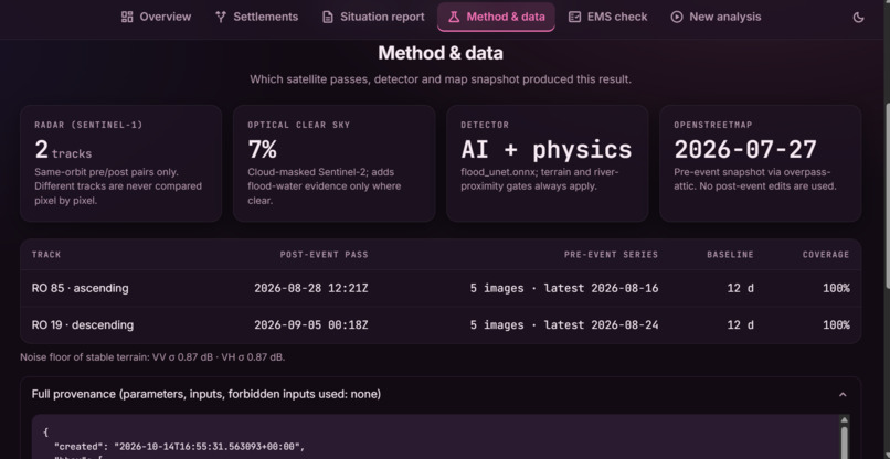
Method and Data
-
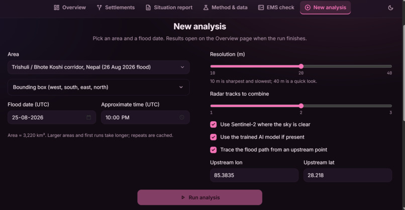
New Analysis
-
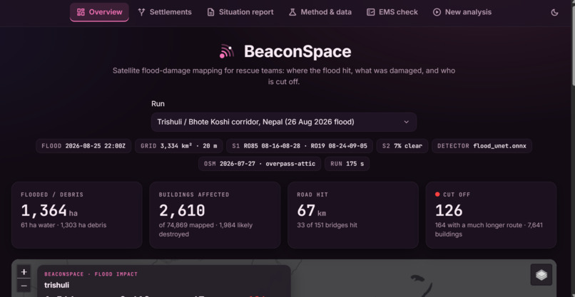
Overview
-
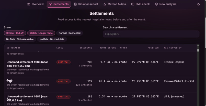
Settlements
-
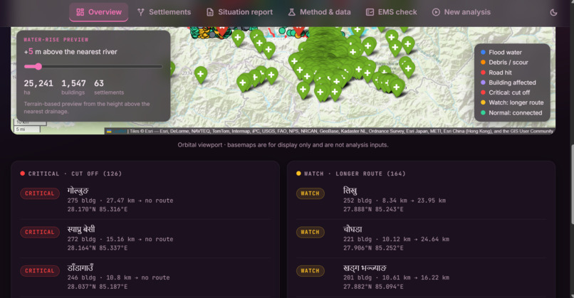
Cutoff and Longer routes
-
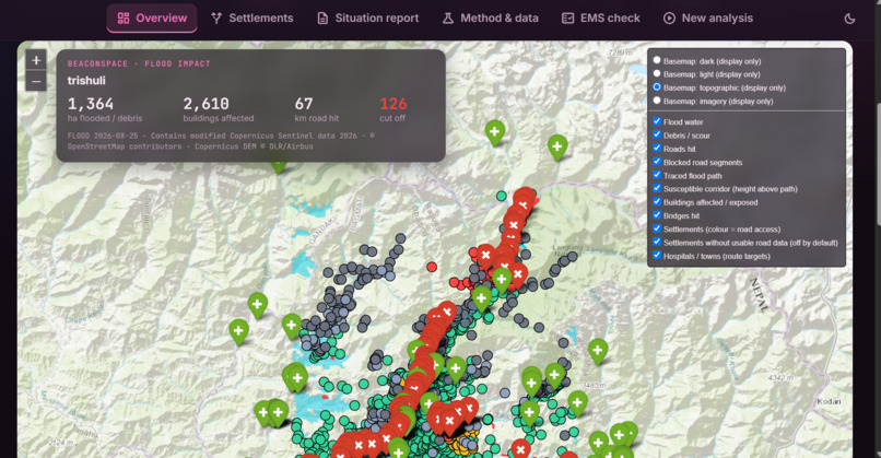
Map
Inspiration
On the night of 25–26 August 2026 a glacial-lake outburst sent a wall of water and debris down the Bhote Koshi and Trishuli valleys in Nepal. In a mountain flood the first things to go are the things that would tell you what happened: gauges are swept away, roads and bridges fail, phone lines drop. The coordinator in Kathmandu is left with the same three questions every time: where did the flood hit, what was damaged, and which villages can no longer be reached?
Satellites keep watching when the ground cannot. Radar sees through monsoon cloud, elevation models tell us where water can go, and OpenStreetMap remembers where the roads and houses were before the event. All of it is free. We wanted to see how far those three ingredients alone could take a rescue team in the first days, and to build something that works for any area and date, not just one hand-tuned example. We called it BeaconSpace.
What it does
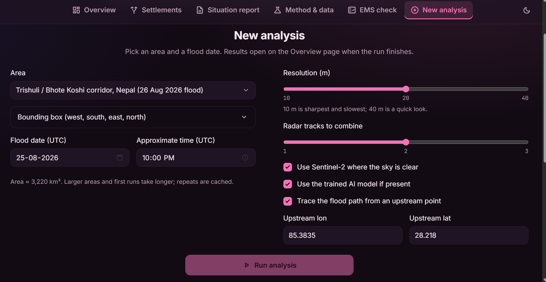
Give it a bounding box and a flood date. It then:
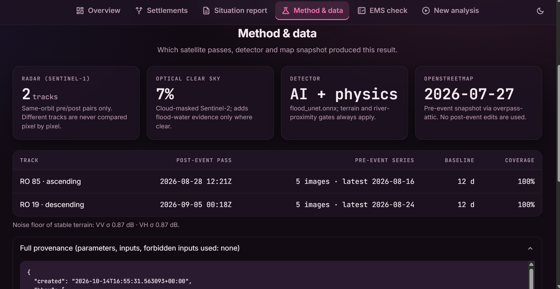
- finds Sentinel-1 radar images from the same orbit track before and after the event, and maps flood water and debris/scour;
- adds Sentinel-2 optical evidence where the sky is clear;
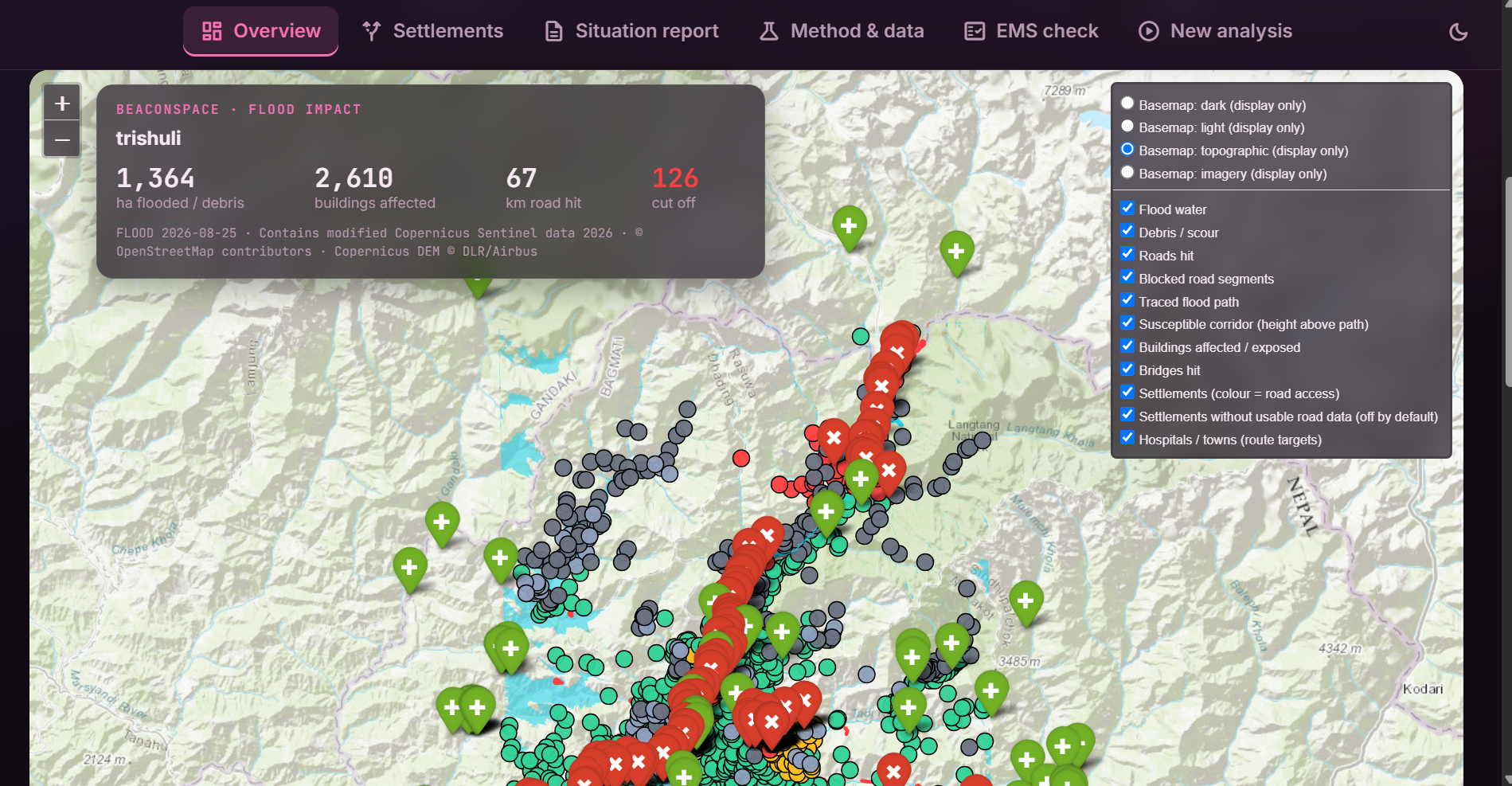
- overlays the OpenStreetMap snapshot from before the event to estimate damaged buildings, roads and bridges;
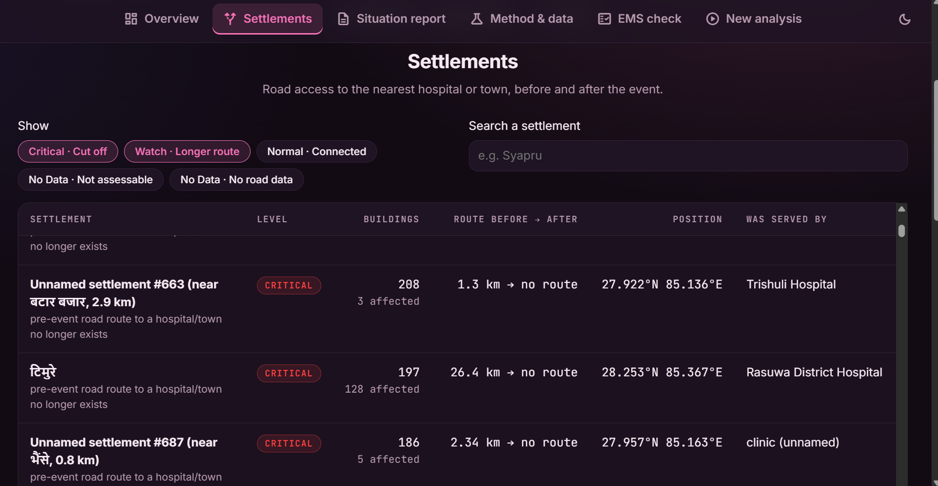
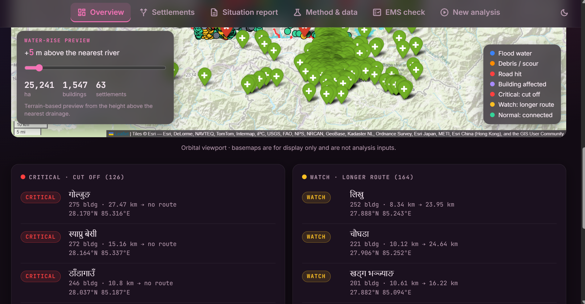
- rebuilds the road graph with flooded segments removed and finds the settlements that lost their route to a hospital or town;
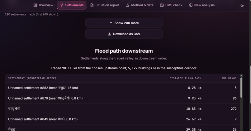
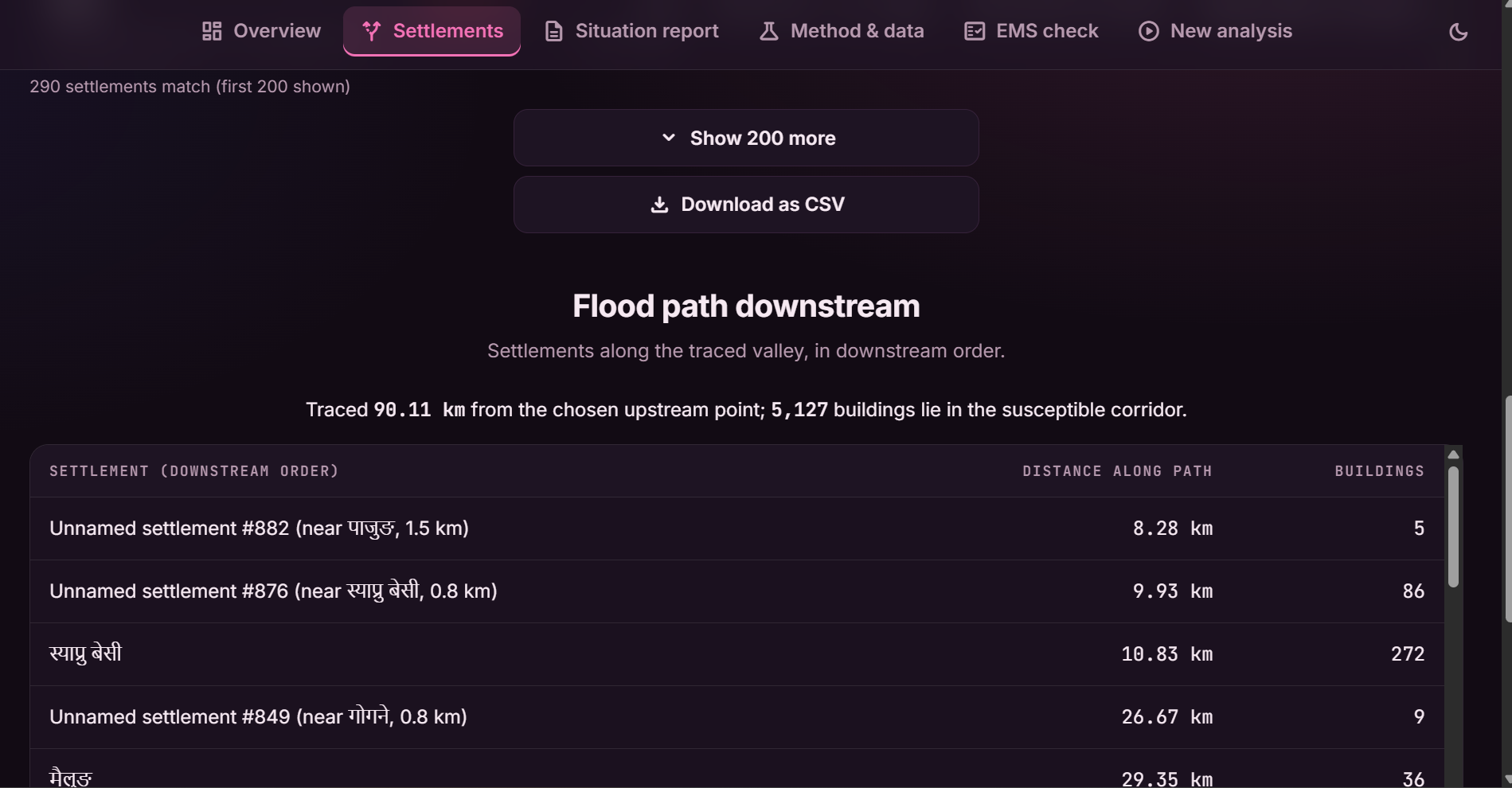
- traces the flood path downstream from an upstream point (bonus) and previews "what if the water rose $h$ metres";
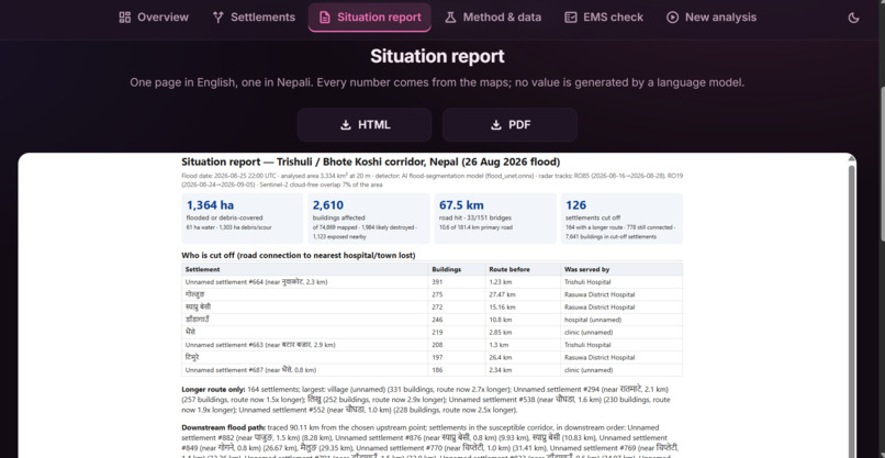
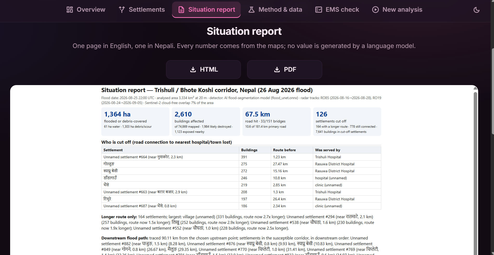
- writes an interactive dashboard and a one-page situation report in English and Nepali, where every number is computed from the maps rather than generated by a language model.
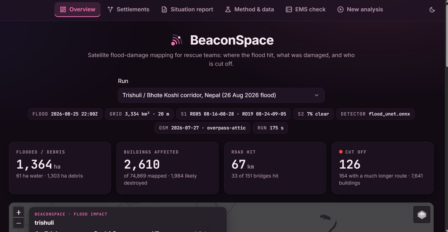
For the Trishuli case study it reports about 1,364 ha of flood and debris, 2,610 affected buildings, 67 km of road and 33 of 151 bridges hit, and 126 cut-off settlements.
How we built it
Radar change detection. Radar backscatter is measured in decibels, so a change is a difference, i.e. a log-ratio. For a pixel we compare the post-event image with the pre-event series on the same relative orbit:
$$\Delta = \sigma^0_{\text{post}} - \sigma^0_{\text{pre}} \quad [\text{dB}], \qquad z = \frac{\bar\Delta}{s_{\text{pre}}}$$
where $\bar\Delta$ is a speckle-smoothed change and $s_{\text{pre}}$ is that pixel's own variability over up to five earlier images. Open water is dark and has just become dark, which separates it from radar shadow (dark in both images):
$$\text{water} \iff \sigma^0_{VV} < T \;\wedge\; \Delta_{VV} \le -3\ \text{dB}$$
Debris and scour are flagged where $z$ is large, but only within 150 m of the drainage network (upstream area $\ge 5\ \text{km}^2$) and on plausible terrain. Terrain comes from the Copernicus DEM: slope, and height above nearest drainage (HAND), which says how far above the river a cell sits. The water-rise preview is simply the set of cells with $\text{HAND} \le h$ connected to the river, and the flow path follows D8 steepest-descent routing.
The AI component. We trained a U-Net with a ResNet-34 encoder on the Kuro Siwo flood dataset, on a free Colab T4. Its seven input channels are post VV/VH, pre VV/VH, the smoothed change in both polarisations, and slope. The feature construction is identical in the training notebook and in the live system (a unit test enforces it), and the trained network is exported to ONNX so the dashboard runs it on a plain CPU.
Who is cut off. Roads from the pre-event OSM snapshot become a graph. A segment is blocked when the flood mask overlaps it enough, and for each settlement we compare the shortest route to a hospital or town before and after:
$$\text{status}=\begin{cases}\text{cut off} & \text{no route after}\ \text{longer route} & d_{\text{after}}/d_{\text{before}} \ge 1.5\ \text{connected} & \text{otherwise}\end{cases}$$
The product. A Python pipeline (floodsys) does the analysis; a FastAPI server exposes it; a React front end (originally Streamlit, rewritten for speed) gives a mission-control style map, settlement tables, the bilingual report, a methods page and the comparison with the official Copernicus EMS maps. Light and dark themes, empty and loading states, and a run form that shows each processing step.
Staying inside the rules. Only allowed inputs are used. A small guard module checks every remote read against the allowed hosts and refuses reference-map paths; the OSM snapshot must predate the event; the official EMSR927 maps are read only by a separate evaluation script, never by the pipeline. Each run records its sources in provenance.json.
What we learned
- A good score on one example proves little. Our first detector matched the official EMS maps well. Then we ran the same detector on image pairs where nothing happened and it flagged 670–2,620 ha of "debris": monsoon farmland changes a lot in radar. That null-event test changed the design. We added per-pixel pre-event variability and the river-proximity rule, which cut false alarms on late-season pairs to 42–71 ha against 880–990 ha for the real event, at the price of some recall.
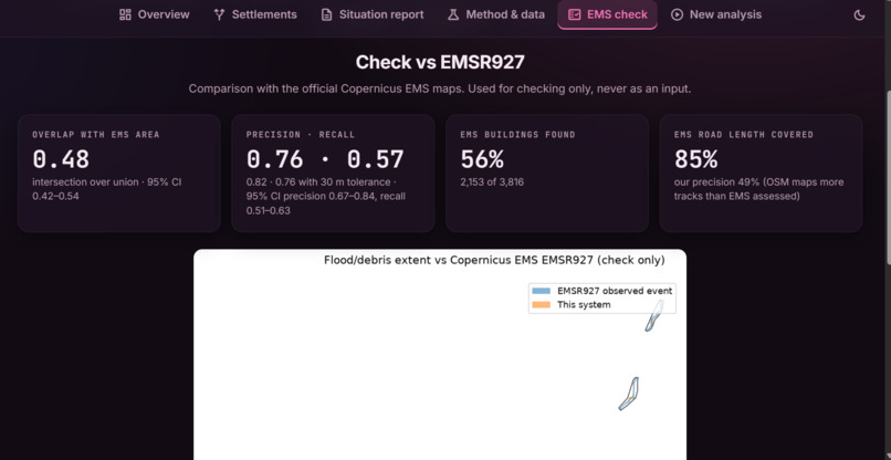
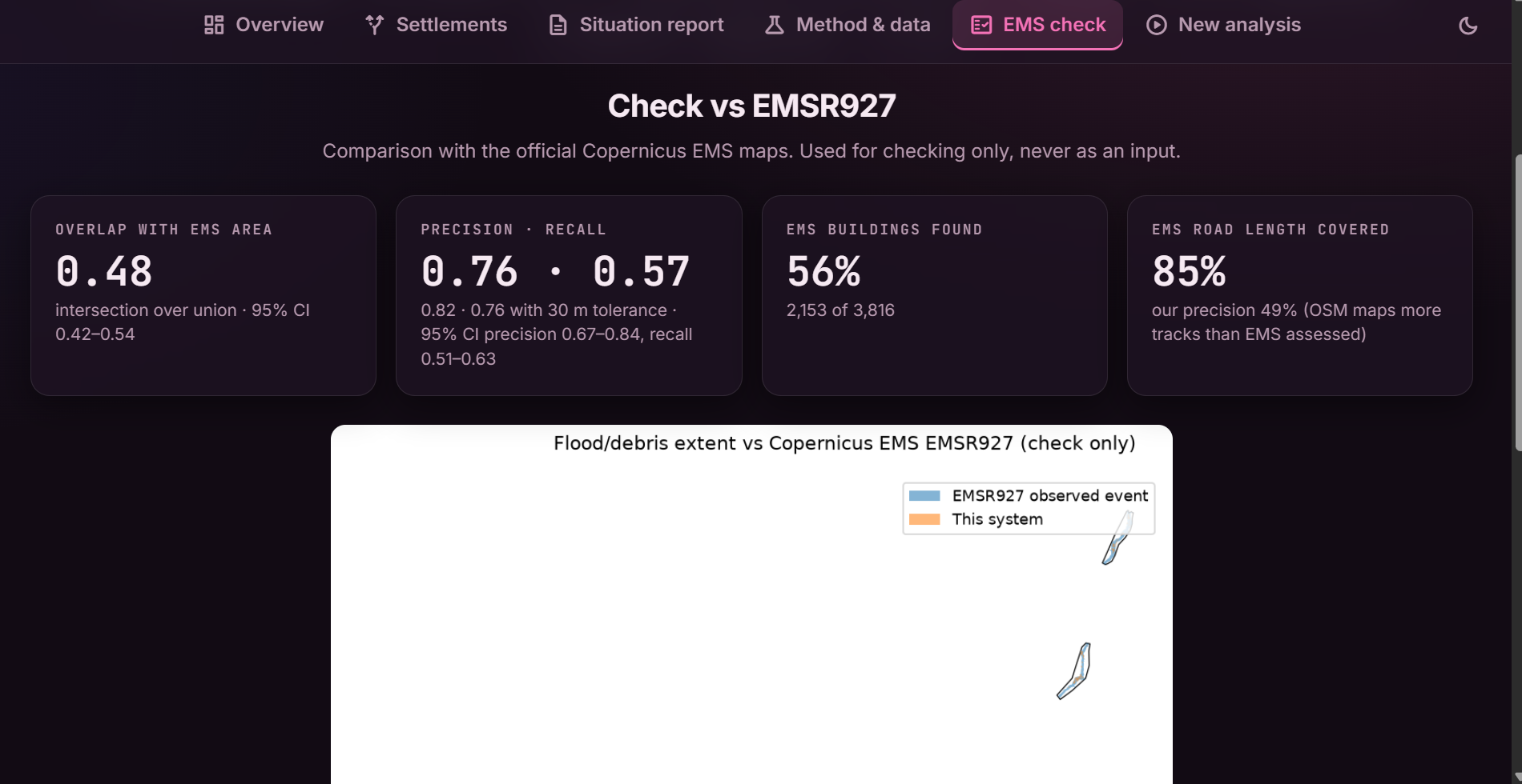
- Measure the uncertainty you are tempted to hide. Against EMSR927, inside the EMS-mapped areas, we get
$$\text{IoU}=\frac{|A\cap B|}{|A\cup B|}=0.48,\quad \text{95\% CI (1 km block bootstrap)}=[0.42,\,0.54]$$
with precision 0.76 and recall 0.57. The cut-off count is also sensitive to our own blocking rule: 126 in the base run, 74–153 across four reasonable rules.
- Check what the AI really adds. The network scores IoU 0.72 across all test-shard patches, but 19 of the 25 test events also occur in training, so that number is optimistic. On the 6 events never seen in training, per-event IoU ranges from 0.15 to 0.92. On the Trishuli debris flow, the network changes the result by only about 1%; the physics-based change detector does the work. The network's measured value is on open-water floods.
- Real data is messy. Open data beats no data, but it comes with access rules, gaps, and surprises we had to design around.
Challenges we faced
- OpenStreetMap history. The ohsome API named in the brief refused our requests (HTTP 403). We built a provider chain that falls back to date-pinned Overpass "attic" queries, with a resumable tile cache and bundled tiles for the case study. It is slow for a brand-new area (tens of minutes to an hour), and that remains the biggest practical limitation.
- Tracks must not be mixed. Different orbit tracks view the terrain from different angles, so pixel comparisons across tracks are invalid. Planning same-track pre/post pairs, and merging detections from two tracks, took more care than the detector itself.
- Shadow, snow and farmland. Radar shadow looks like water, wet snow looks like change, and monsoon fields shimmer. Each needed its own gate (the 3 dB drop rule, terrain gates, the river-proximity rule).
- Almost no optical data. Only about 7% of Sentinel-2 pixels were clear in the monsoon, so optical evidence stays strictly additive and radar leads.
- Honest evaluation. We had to correct our own evaluation twice: once for the train/test event overlap, and once after the null-event test. It was uncomfortable and worth it.
- Limits we state openly. Debris is detected as change near rivers, not classified; hill-slope landslides far from rivers are out of scope; satellites revisit every few days, so the maps show the scene at the post-event pass; and the cut-off analysis only knows mapped roads. The Nepali text is template-based and needs review by a native speaker.
What's next
Same-season baselines to remove the early-monsoon false alarms, faster OpenStreetMap access, debris-flow labels to train the network where it matters, SAR coherence to separate scoured from changed surfaces, per-pixel uncertainty maps, and a native-speaker review of the Nepali report.
Built With
- fastapi
- folium
- geopandas
- google-colab
- javascript
- leaflet.js
- networkx
- numpy
- onnx
- onnx-runtime
- openstreetmap
- pyflwdir
- python
- pytorch
- rasterio
- react
- scikit-image
- scipy
- segmentation-models-pytorch
- sentinel-1
- sentinel-2
- shapely
- uvicorn
- vite

Log in or sign up for Devpost to join the conversation.