AquaSense Water Intelligence for a More Resilient Future.
AquaSense is a global water intelligence platform that turns open satellite and hydrological data into an interactive geospatial workspace. Explore anywhere on Earth, draw and save your own study regions, then open a dedicated analytics view that computes real water indicators for that exact polygon — with every value carrying its source, date, resolution and data status.
Source Code
AquaSense Earth Explorer — globe with a drawn region
The Inspiration Water is one of the most important resources on the planet, yet understanding water conditions across different regions is surprisingly hard.
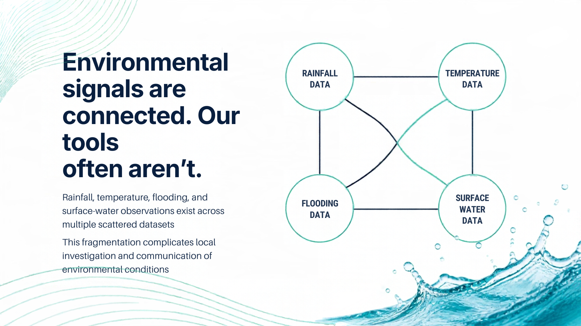
Satellite surface-water archives, rainfall reanalysis, river-discharge models and scene catalogues live on different platforms, in different formats, at different resolutions. Even when you can reach the data, knowing what it means requires context.
A rainfall deficit does not prove water scarcity. Heavy rainfall does not mean a flood occurred. A water-occurrence percentage is a frequency, not a volume. A modelled discharge estimate is not a gauge reading.
That led to one question:
What if you could investigate water conditions anywhere on Earth through one workspace — and understand not only what the data shows, but where it came from, how it was processed, and what it cannot establish?
AquaSense is our answer.
The Problem 🌍 Fragmented environmental data — investigating one location means juggling several providers and mapping tools. 📊 No spatial control — most tools give you a point or a city. Real water analysis needs your boundary: a lake, a reservoir, a river reach, a watershed. 🌦️ Confusing data classifications — reanalysis, forecasts, modelled estimates and observations are different kinds of evidence. 🔎 Invisible coverage gaps — a missing value must never look like a normal one. 🛰️ Disconnected satellite information — finding available scenes usually means leaving the map for a separate catalogue search. 🎯 Unsupported conclusions — environmental data misleads when its limits are not stated. The Solution One workflow: draw an area, name it, save it, and analyse the real data inside that exact polygon.
Explore a Worldwide Globe Search any place or paste coordinates, then explore on a MapLibre GL globe with satellite imagery, or switch to a flat map. A raster slippy-map fallback with real Web Mercator keeps navigation working where WebGL2 is unavailable.
Draw and Save Your Own Regions Pick the Draw an area tool and click the map to place vertices. Enter finishes the ring, Escape cancels, Backspace removes the last point. The ring is validated server-side — self-intersection, size limits and geodesic area — before anything is created. Name it, choose a region type and water feature, pick a colour, and save. You stay on the map, with the new region selected and highlighted.
Manage Regions in a Shared List A right-side Region List rail appears on both the map and analytics surfaces, backed by the real saved regions. Search, filter, sort, rename, recolour, edit the boundary, delete, or open analytics.
Open Real Per-Region Analytics Everything is computed from the actual polygon, not a point guess.
Surface water — extent, mean / median / p90 water-occurrence and mean seasonality in months, from the JRC Global Surface Water 30 m archive (1984–2021). Rainfall and temperature — daily and total precipitation plus mean / max / min temperature from ERA5 via Open-Meteo, drawn as bar and max–min line charts. River flow — modelled discharge and forecast from Open-Meteo Flood (GloFAS), explicitly labelled modelled, not gauged. Water quality and water stress — shown as Unavailable, with the reason, because we will not fabricate a number we cannot source.
Explore Satellite Imagery and Scenes Toggle key-free NASA GIBS WMTS layers — IMERG precipitation, MODIS combined flood (MCDWD), MODIS land-surface temperature, MODIS NDVI, HLS S30/L30, OPERA dynamic surface-water extent and true colour. Each layer is probed live and unserved ones are greyed with a reason. Search the Copernicus CDSE STAC and NASA HLS (CMR STAC) catalogues for scene metadata, footprints and acquisition dates.
Keep Provenance on Every Value Every metric carries a value, unit, source, observation date or period, spatial and temporal resolution, processing method and a status — Observed, Derived, Estimated, Forecast, Demo or Unavailable.
The Science The analysis is not a lookup table. Here is what the backend actually computes.
Geodesic polygon area uses the spherical-excess method with the mean Earth radius ( R = 6371.0088 ) km:
$$A = \left| \frac{R^2}{2} \sum_{i} \Delta\lambda_i \left( 2 + \sin\varphi_i + \sin\varphi_{i+1} \right) \right|$$
where ( \varphi ) is latitude and ( \lambda ) is longitude in radians. This is why a drawn area reports a real square-kilometre value rather than a pixel count.
Rainfall anomaly compares the observed total ( O ) against a compatible baseline ( B ) over the same calendar window:
$$\text{anomaly}\text{mm} = O - B \qquad \text{anomaly}{%} = \frac{O - B}{B} \times 100$$
The percentage is only produced when ( B > 0 ), and the deficit / excess band is labelled a preliminary AquaSense indicator, not a water-scarcity verdict.
Water occurrence is decoded from the JRC archive's blue channel and reduced over only the pixels inside your ring:
$$\text{occurrence}_{%} = \frac{\text{blue}}{255} \times 100$$
Seasonality is decoded from the dataset's 12-class ramp into months-present. NoData is excluded, and the source's 30 m resolution is preserved.
How We Built It The frontend visualises the evidence. Python does the analysis. Data provenance explains what the results mean.
             ┌────────────────────────┐
             │          User          │
             └────────────┬───────────┘
                          │
                          ▼
             ┌────────────────────────┐
             │     Next.js 14 App     │
             │ React · TypeScript     │
             │ Tailwind · MapLibre    │
             │ ECharts · Zod          │
             └────────────┬───────────┘
                          │
                same-origin /api/* proxy
                          │
                          ▼
             ┌────────────────────────┐
             │     FastAPI Backend    │
             │ Python · Pydantic v2   │
             │ HTTPX · NumPy · Pillow │
             └────────────┬───────────┘
                          │
          ┌───────────────┼────────────────┐
          ▼               ▼                ▼
   ┌────────────┐  ┌─────────────┐  ┌─────────────┐
   │  Provider  │  │  Analysis   │  │ Provenance  │
   │  Adapters  │  │  Services   │  │   Models    │
   └─────┬──────┘  └─────────────┘  └─────────────┘
         │
┌─────┬───┴────┬───────────┬───────────┐ ▼ ▼ ▼ ▼ ▼ JRC Open- NASA Copernicus Geocoding / GSW Meteo GIBS/POWER / CDSE STAC OSM Frontend
Next.js 14 with the App Router, React 18, TypeScript in strict mode Tailwind CSS for the design system MapLibre GL for the globe and flat map ECharts for every chart Zod for runtime response validation Backend
FastAPI with Pydantic v2 models and HTTPX for async provider calls NumPy and Pillow for raster decoding and polygon statistics reportlab for PDF reports pytest and respx for testing 35 REST endpoints across 11 routers. Provider adapters isolate every external service; analysis services handle geometry validation, geodesic area, raster reduction, temporal aggregation and location summaries.
Real data sources connected
JRC Global Surface Water (30 m) — water extent, occurrence, seasonality ERA5 via Open-Meteo — historical rainfall and temperature Open-Meteo Flood (GloFAS) — modelled river discharge and forecast NASA GIBS WMTS — IMERG, MCDWD flood, MODIS LST/NDVI, HLS, OPERA DSWx, true colour Copernicus CDSE STAC — satellite scene metadata and previews NASA HLS (CMR STAC) — HLS granule search NASA POWER — independent reanalysis cross-check NASA GPM IMERG Late Daily V07 — satellite precipitation (optional Earthdata login) Open-Meteo Geocoding (GeoNames) — global place search OpenStreetMap (Overpass) — water-body features Reliability. The browser talks to a same-origin API proxy implemented as a Next.js route handler, so backend configuration never reaches the client — and an unreachable backend returns a structured 503 instead of a bare error. The analysis layer checks completeness and compatibility before producing comparisons. Regions persist in a JSON-file-backed store, which is the right level of complexity at this stage.
Challenges We Ran Into Turning a raster archive into per-polygon statistics. JRC Global Surface Water is a 30 m global raster. To report it for your polygon we decode its public PNG tiles, map pixel coordinates back to geography, and reduce only the pixels inside the ring with NumPy — accounting for NoData and preserving resolution. Doing this in the browser would have been unreliable.
Keeping scientific meaning intact. Occurrence is a frequency, not a volume. Discharge is modelled, not gauged. IMERG is satellite-estimated, not a rain gauge. The data model carries a status on every metric so the interface can never blur these together.
Producing defensible comparisons. An anomaly is only meaningful when periods are compatible, so comparisons are gated on complete, same-length series.
Handling missing coverage honestly. Water quality and water stress have no connected source, so AquaSense says Unavailable with the reason instead of inventing a score. GRACE storage is scale-gated because its ( \sim 300 ) km footprint cannot speak to a small lake.
A resilient map. The globe needs a WebGL2 context that is not guaranteed, so a separate raster slippy-map keeps navigation and selection alive without it.
Getting the workflow right. Our first pass auto-opened analytics the moment you saved a region — which threw you out of the map mid-investigation. We changed it so saving keeps you on the map with the region highlighted, and pinned that behaviour with a test.
Accomplishments We're Proud Of 🌍 A worldwide globe with a non-WebGL fallback. ✏️ Real polygon drawing with Enter / Escape / Backspace, server-side validation and geodesic area. 💾 Persistent saved regions with a full shared Region List. 📈 Per-region analytics computed from the actual polygon, not a point guess. 🌊 Real integration with JRC Global Surface Water at 30 m, reduced with NumPy inside the ring. 🌦️ History and forecast kept strictly separate. 🛰️ Two live scene catalogues plus seven GIBS raster layers, each probed at runtime. 🧾 A consistent provenance model across every metric. 🧪 202 backend tests (200 passing, 2 skipped) and 140 frontend tests across 26 files. 🛡️ A product that treats the reliability of the data as part of the feature set. What We Learned Provenance is product, not paperwork. Users need to know where a number came from to trust it. Classification changes interpretation. Reanalysis, forecast and model output are not observations. A boundary is the unit of water analysis. A city centroid cannot answer a reservoir question. Validation prevents false confidence. Incomplete data should not produce a tidy chart. Honesty is a feature. Saying "unavailable" is more valuable than a plausible invention. Current Limitations AquaSense is a global water-intelligence workspace, not a dedicated flood-prediction or satellite change-detection system.
Surface water is the JRC 1984–2021 archive, not a live feed. Occurrence is a frequency, not a volume. River discharge is modelled (GloFAS) at a model point, not gauged across the polygon. Water quality and water stress are unavailable — no source is connected, so we say so. GRACE storage is coarse and only shown where the region is large enough to be meaningful. IMERG satellite precipitation needs optional Earthdata credentials; it reports unconfigured rather than pretending. Persistence is a JSON-file store, appropriate now but not multi-user. We document these boundaries because environmental software should never claim more certainty than its implementation supports.
What's Next 🗄️ Migrate region persistence to PostGIS for spatial queries and multi-user use. 🌧️ Add versioned historical baselines through Copernicus CDS. ⚡ Introduce bounded caching keyed on dataset, geometry hash and date range. 🛰️ Connect a validated satellite surface-water change-detection pipeline. 📍 Integrate a well-documented regional gauge network. Water-body change detection and dedicated flood prediction remain future work, not completed features.
Final Thought Water challenges are complex. Understanding them takes more than a single rainfall value, a forecast, or a map. It takes context, real evidence, and transparency about what the data can actually establish.
Draw the area. See the evidence. Know its limits.
AquaSense — Water Intelligence for a More Resilient Future.
Built With
- climate-change
- copernicus-data-space-ecosystem
- data-visualization
- echarts
- environmental-sustainability
- fastapi
- geospatial
- httpx
- javascript
- maplibre-gl
- nasa-power
- next.js
- open-meteo-api
- openstreetmap
- pydantic
- pytest
- python
- react
- rest-api
- tailwind-css
- typescript
- water-management
- zod


