zoning-ca

• 

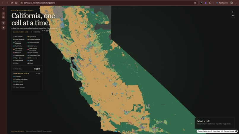
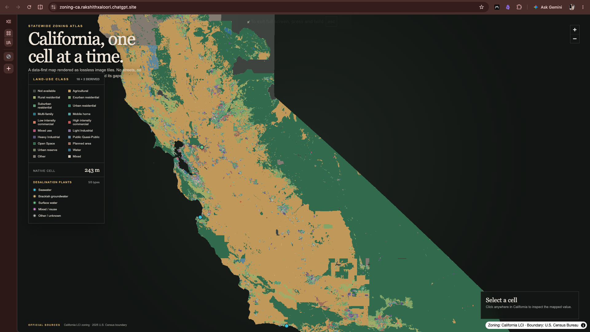
  California's zoning map with plotted desalination plants

Inspiration

California has sunlight, seawater, land, infrastructure, and enormous demand for industrial chemicals. It also has desalination plants that produce concentrated brine—material that is usually treated as a disposal problem.

Bipolar-membrane electrodialysis offers a more interesting possibility. Using ion-selective and bipolar membranes, a plant can convert sodium chloride recovered from desalination brine into sodium hydroxide and hydrochloric acid. Electricity is the principal process input. Put the plant near a source of brine, give it access to inexpensive solar power, and a waste stream begins to look like an industrial resource.

The chemistry is straightforward:

$$ \mathrm{NaCl} + \mathrm{H_2O} \xrightarrow{\text{bipolar-membrane electrodialysis}} \mathrm{NaOH} + \mathrm{HCl} $$

The geography is not.

A viable site needs compatible zoning, proximity to a desalination facility, enough nearby agricultural or open land for solar generation, and eventually access to power, transportation, water, customers for both products, and safe acid-and-base handling infrastructure. The relevant information exists, but it is scattered across incompatible datasets and hundreds of local jurisdictions.

We built zoning-ca to make the first cut.

What it does

zoning-ca turns California’s fragmented zoning record into a single interactive land-use map. The state is represented as a grid of approximately 250-meter cells, each classified by its dominant land use.

On top of this grid, we plot desalination plants and distinguish them by water source: seawater, brackish groundwater, surface water, mixed or reused water, and other sources.

With one map, a user can:

• Scan the entire state for industrially zoned areas.
• Find agricultural and open-space land that may accommodate solar generation.
• Compare those areas with the locations of desalination plants.
• Filter desalination facilities by water source.
• Inspect plant capacity, operator, status, and provenance.
• Click any mapped cell to retrieve its land-use class and coordinates.

This does not produce a permit-ready plant location. It does something more appropriate for the available data: it reduces a state of 164,000 square miles to a tractable set of places worth investigating.

How we built it

The raw material is California’s official statewide zoning dataset, published in separate northern and southern layers by the California Office of Land Use and Climate Innovation.

Together, the layers contain:

• 568,741 zoning polygons.
• 534 unique jurisdictions.
• 18 normalized statewide land-use classes.
• Roughly 800 MB of compressed source data.

Sending half a million polygons to a browser would be slow, memory-intensive, and unnecessary. Site screening does not require every parcel boundary at every zoom level. It requires a consistent statewide representation that preserves the land-use signal.

We therefore converted the polygons into a raster grid aligned with standard Web Mercator map tiles. At zoom level 9, each pixel represents about 243 meters on the ground near the center of California—close to our 250-meter target.

Each cell is sampled on a (4 \times 4) subgrid:

$$ N_{\text{samples}} = 4 \times 4 = 16 $$

If more than half of those samples belong to one zoning class, that class wins. If zoning is present but no class has a majority, the cell is labeled Mixed. A cell inside the official California boundary with no zoning coverage is labeled Not available. Everything outside the state is transparent.

The classified grid is converted into a multiresolution pyramid of lossless PNG tiles. The browser downloads only the tiles currently visible on screen, not the underlying polygon dataset.

The interface is built with React, Next.js, TypeScript, and MapLibre GL. Zoning is rendered as a raster source. Desalination plants are loaded from GeoJSON as a lightweight interactive overlay.

The result is simple in the browser because the expensive decisions have already been made during preprocessing.

Challenges we ran into

The first challenge was semantic, not computational. California does not have one zoning system. It has hundreds of them. The same practical land use may be described by different codes, abbreviations, and local planning conventions in every jurisdiction.

The second challenge was scale. The source data contains 568,741 geometries, some highly detailed. Rendering all of them directly would make statewide exploration sluggish and would transfer far more information than the user needs.

The third challenge was preserving ambiguity. A cell can cross several parcels or zoning classes. Assigning the class found at its center would be fast but misleading. Sampling each cell 16 times gave us a practical measure of dominance while retaining a distinct Mixed category for genuine boundaries.

We also had to:

• Reproject datasets supplied in different coordinate systems.
• Join northern and southern zoning layers without losing statewide consistency.
• Clip the output against an authoritative California boundary.
• Separate missing zoning coverage from territory outside the state.
• Normalize inconsistent descriptions of desalination water sources.
• Preserve traceable sources for every desalination facility.
• Keep the application responsive without concealing uncertainty in the data.

Finally, zoning is not permission. The statewide dataset is useful for screening, but any real project would still require verification against current local ordinances, overlays, environmental rules, parcel conditions, and permitting requirements.

Accomplishments that we're proud of

We compressed an unwieldy statewide planning dataset into a map that loads quickly, reads clearly, and remains honest about gaps and mixed classifications.

The architecture scales because it moves complexity out of the browser. Whether the source contains ten thousand polygons or half a million, the browser still sees ordinary 256-pixel image tiles.

We are also proud that the map connects land-use planning to a concrete industrial question. A zoning atlas is informative. A zoning atlas combined with desalination infrastructure begins to reveal supply chains.

Most importantly, the project establishes a reproducible foundation. The inputs, checksums, classification method, grid resolution, and derived categories are documented. The result can be rebuilt rather than merely viewed.

What we learned

Industrial development is an exercise in constraint intersection.

No single variable identifies a good site. Cheap land is irrelevant if it cannot be used for industry. Industrial zoning is insufficient without feedstock. Brine is not useful without energy. Solar potential does not matter without enough land or grid access. A location that satisfies every technical requirement can still fail on environmental, logistical, or political grounds.

We also learned that resolution should follow the decision being made. Parcel-perfect geometry is necessary for permitting. It is unnecessary for asking which regions of California deserve closer study. At the screening stage, a consistent 250-meter approximation is often more useful than an inconsistent collection of extremely detailed local maps.

Finally, missing data is itself data. Showing Not available is better than filling gaps with false certainty.

What's next for zoning-ca

The current map answers a qualitative question: where do promising combinations of zoning and desalination infrastructure appear?

The next version should answer a quantitative one: which candidate sites survive all of the important constraints?

We plan to add:

• Travel and straight-line distance to desalination plants.
• Brine production volume, salinity, ion composition, pretreatment requirements, and availability.
• Nearby demand for sodium hydroxide and hydrochloric acid.
• Industrial parcel identification and minimum contiguous-area requirements.
• Solar irradiance, developable acreage, and estimated annual generation.
• Grid substations, transmission capacity, and electricity-price signals.
• Highway, rail, port, pipeline, and customer access.
• Water constraints, protected habitats, flood risk, seismic risk, and environmental-justice indicators.
• Explicit exclusion rules for physically or legally infeasible sites.
• Ranked candidates with complete, inspectable score breakdowns.

A first-pass suitability model might look like:

$$ Q = w_bB + w_zZ + w_sS + w_gG + w_tT - w_eE - w_rR $$

where:

• (B) measures access to usable brine.
• (Z) measures zoning compatibility.
• (S) measures solar-generation potential.
• (G) measures grid access.
• (T) measures transportation and customer access.
• (E) measures environmental constraints.
• (R) measures development and permitting risk.

The score itself is not the product. The valuable part is making every assumption visible: what was measured, how it was normalized, why it was weighted, and which constraint eliminated a site.

California already contains the necessary physical ingredients. zoning-ca is an attempt to assemble the geographic evidence and determine where those ingredients can actually be combined.

Built With

• codex