-
-
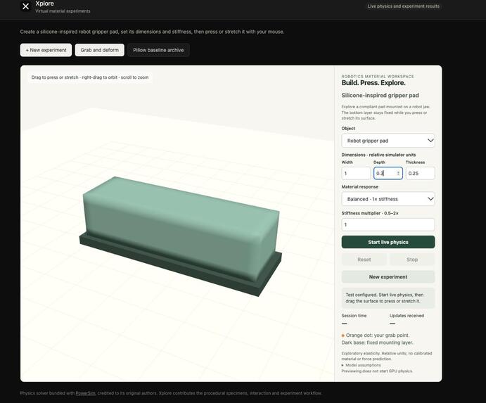
Basic Interface of X object.
Inspiration
Every soft robotic gripper touches the world through a silicone pad, and the pad's stiffness can make or break the gripper. If the pad is too soft, it squashes under load and the grip loses precision. If it's too firm, it can't conform to delicate or irregular parts.
Most small robotics teams still choose that stiffness by trial and error. They design a mould, mix and cast the silicone, wait hours for it to cure, test it, and start again. Every round costs time and money, and the reason one pad beat another is rarely written down.
Research-grade soft-body simulators can already model this kind of deformation, but they live in scripts, config files and GPU clusters. We wanted to put one behind a workflow a design team can actually use, so they can test the pad before they cast it.
What it does
Xplore is a virtual test bench for choosing the stiffness of a silicone gripper pad.
Set up the comparison. Pick up to three stiffness options for the same pad (Flexible, Balanced and Firm), set the maximum compression your design can tolerate, and optionally enter what each prototype would cost you.
Run identical experiments. Xplore runs the same GPU physics experiment on each option. Geometry, supports, load, duration and numerical settings are identical. Only stiffness changes: each option uses the baseline stiffness multiplied by 0.5, 1 or 2.
Compare the results. You get synchronised simulation videos, a compression-over-time chart and a comparison table.
Get a shortlist with reasons. A deterministic rule shortlists the options that meet your limit and highlights the cheapest one to cast next, when costs are available for every qualifying option, along with a plain-language explanation and a suggested next physical test.
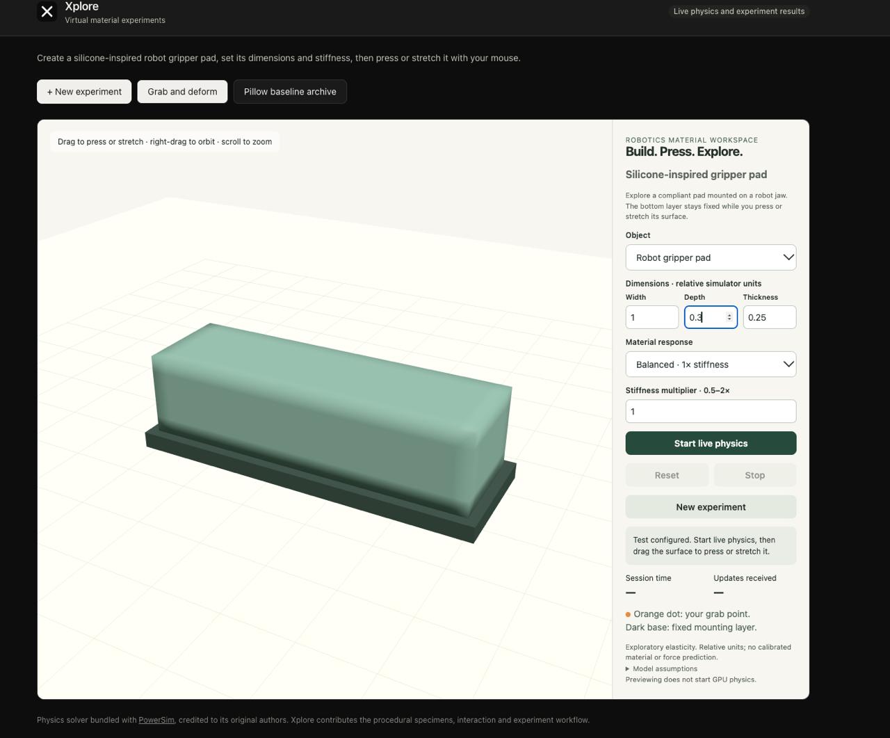
Grab and deform. Press and pull the pad with your mouse while a GPU physics solver streams the deformation live.
The stiffness options. For option k, we scale the baseline Young's modulus E_0:
E_k = s_k × E_0

Flexible: s_k = 0.5
Balanced: s_k = 1
Firm:     s_k = 2
The measurement. Before any load is applied, we fix the membership of two particle groups, U (upper) and L (lower). For each group, we calculate its centroid:
centroid_G(t) = sum of particle positions in G at time t
                / number of particles in G

G is either U or L.
We track the separation of these centroids along a fixed unit loading axis n_hat, oriented so the initial separation is positive:
d(t) = dot(centroid_U(t) - centroid_L(t), n_hat)

d_0 = d(0) > 0
Here, dot is the vector dot product, so d(t) measures separation along the loading axis.
Compression is the relative loss of that separation, expressed as a percentage. We report its peak over a fixed window from 0 to T, using the same window for every option:
c(t) = 100 × (d_0 - d(t)) / d_0

c_peak = maximum value of c(t) over 0 ≤ t ≤ T
The shortlist rule. Given your compression limit c_max, expressed on the same percentage scale, the qualifying set is:
Q = {option k for which c_peak,k ≤ c_max}
For example, a limit of 10 means a maximum compression of 10%.
If Q is nonempty and every qualifying option has a prototype cost p_k, Xplore selects a recommendation using these priorities, in order:
- Lowest prototype cost.
- Lowest peak compression, if costs are tied.
- Stable option ID, if both cost and compression are tied.
Recommended option = lexicographic minimum over Q of:

(prototype cost, peak compression, stable option ID)
If nothing qualifies, Xplore says so and suggests a bounded follow-up instead of inventing a winner. If any run failed, or the numerics are sensitive, the shortlist is marked provisional.
Every comparison is saved as a reproducible record: inputs, measurements, engine version, config hash and evidence status. You can reopen any record from its URL. Identical physics inputs hit a cache, so changing only the limit or the costs re-ranks the options in seconds.
How we built it
- Contract first. In the first hour we wrote and froze a JSON Schema for the API, along with example fixtures. The frontend was built against a mock API while the GPU pipeline came up, and the real backend later plugged in with no schema changes.
- Simulation. We used PowerSim at a pinned upstream commit, running Python 3.11, CUDA 12.8 and PyTorch on NVIDIA GPUs on Modal. We wrote a small export adapter so each run saves an unloaded baseline, stable particle IDs and float32 positions; metrics are computed in float64.
- Backend. A FastAPI service on Modal handles input validation (before any GPU work), durable job state, persistent artifacts on a Modal Volume, cache keys built from every simulation-relevant input and version, and browser-ready H.264 videos with byte-range support.
- Live interaction. A WebSocket streams solver particle positions to a Three.js surface in the browser. Mouse grabs become velocity constraints on nearby particles. Sessions are bounded in time and count.
- Frontend. React, TypeScript, Vite and Tailwind. Experiments are polled every 2 seconds, survive a page refresh, and show live/cached and evidence labels everywhere. The chart has a crosshair readout and a table view, and the colour palette was checked for colour-blind safety. Headless-browser tests cover every job state: queued, running, completed, partial and failed.
- Cost control. We ran one GPU worker at a time with hard timeouts and capped live sessions. The whole build used about USD 1.25 of Modal compute at our last snapshot.
Challenges we ran into
- No ready-made test. The released scene we started from was a gravity drop, not a controlled compression test. We had to design one ourselves: isolate the object, fix a support group, apply a load pulse with gravity off, and observe over a fixed window. Then we moved the workflow onto the gripper pad.
- Measuring precisely enough. The upstream export writes half-precision positions after stepping, which is too coarse for a percentage metric. We patched in our own export of the unloaded baseline and float32 positions.
- Numerical sensitivity. When we halved the timestep in our first controlled scene, the peak compression changed by 11.8%, missing our 5% convergence goal (see the check below). Instead of hiding it, Xplore shows it and marks the shortlist provisional.
- GPU cold starts and budget. Live sessions need about a minute to allocate a GPU and compile kernels, so we capped sessions, cached compiled kernels and set hard limits.
- Keeping the interface honest. The UI never shows placeholder numbers. Fixtures are labelled illustrative, and cached runs are labelled cached.
- Scope. We cut an AI voice assistant and the saving of live gestures so we could finish a core we trust.
Our convergence check. We rerun the same option with half the timestep and compare the peak compression:
c_coarse = peak compression using timestep dt

c_fine = peak compression using timestep dt / 2

relative difference = abs(c_coarse - c_fine) / abs(c_coarse)
Here, abs means absolute value. This relative measure requires a nonzero reference value c_coarse.
Our goal is a relative difference of at most 0.05 (5%). Our first controlled scene measured approximately 0.118 (11.8%).
Accomplishments that we're proud of
- A real end-to-end pipeline: browser → GPU soft-body simulation → measured metric → deterministic shortlist, on a deployed API.
- Live grab-and-deform of a soft object, driven by real GPU physics, inside a web page.
- Reproducibility. Every result carries its inputs, versions and config hash, and cached comparisons return in seconds.
- Two people building in parallel from minute one, thanks to a frozen contract, with no breaking changes at integration.
- Evidence labels on every result, so a judge or an engineer can see exactly what is and isn't proven.
What we learned
- A simulator isn't a product. The value is in the workflow: fixed definitions, identical conditions and traceable records.
- Formulas run out fast. A textbook formula (below) only covers a simple block. Real gripper pads have shaped geometry, contact, large deformations and dynamic loads, which is why you need simulation, and simulation in turn needs convergence checks.
- Define the metric before you compare. Particle groups, loading axis and aggregation window must be frozen before the first run, or the comparison means nothing.
- Agreeing the contract first saves hours of integration work.
- Saying what you haven't proven builds trust.
Why not just a formula? For a uniform block under uniaxial loading in the small-strain, linear-elastic regime, the magnitude of strain is approximately:
strain ≈ F / (A × E)
Here, F is the applied force magnitude, A is the loaded cross-sectional area and E is Young's modulus.
Under those assumptions, doubling the stiffness would halve the deformation. A real pad generally won't follow that rule exactly.
What's next for Xplore
- Physical validation. Cast pads in two or three silicone hardnesses, calibrate on one load, predict a second load we held back, and report the error.
- Real materials. Map the stiffness options to sourced silicone grades, with proper units.
- Converged numerics. Use finer timesteps and resolution until the convergence checks pass.
- Gripper-specific metrics. Contact area, contact pressure, holding force, slip, recovery and repeated loading.
- Your own pad geometry. Upload a pad design from CAD or a 3D scan.
- Saved interactions and grounded explanations. Record live gestures as experiments, and add an assistant that explains each saved experiment from its record.
