-
-

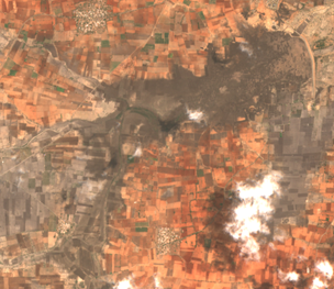
Malavi dam in 29 Oct 2017. One of its peak capacities.
-

Dried up Malavi dam on 27 May 2017.
-

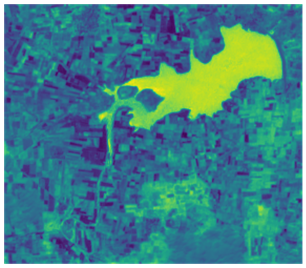
Malavi Dam NDMI on 29 Oct 2017. The brighter the colour the more the moisture, the darker the colour less so.
-
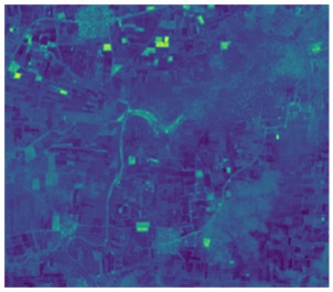
NDMI of dried up Malavi Dam on 27 May 2017. The brighter the colour the more the moisture, the darker the colour less so.
-
NDMI of dried up Malavi Dam on 27 May 2017. The brighter the colour the more the moisture, the darker the colour less so.
-

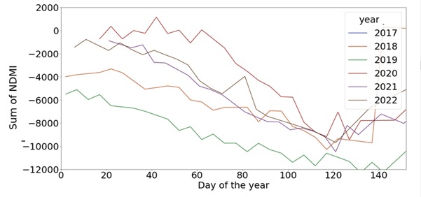
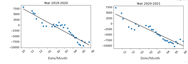
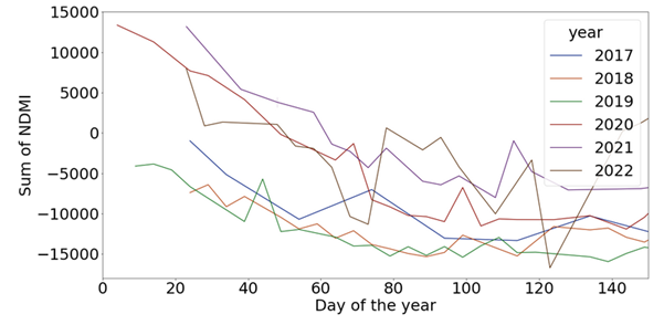
Linear Regression of NDMI sum from Oct 1 to June 1 in the given years for Malavi Dam.
-
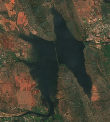
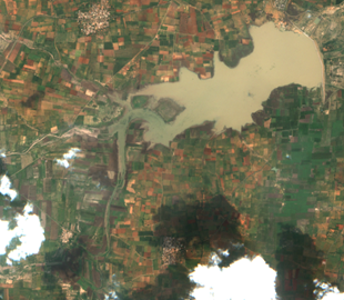
Gandipalem Reservoir on 2022 Feb 2
-
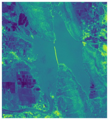
NDMI sum of Gandipalem Reservoir on 2022 Feb 2. The brighter the colour the more the moisture, the darker the colour less so.
-
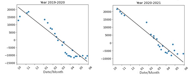
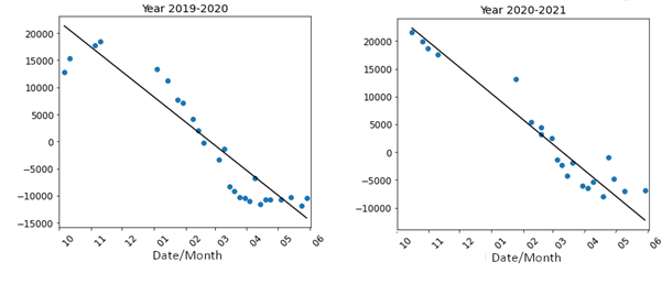
Linear Regression of NDMI sum from Oct 1 to June 1 in the given years n case of Gandipalem reservoir.
-
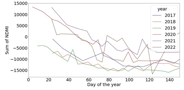
Trend in sum of NDMI over the years for the period from Jan to June
-
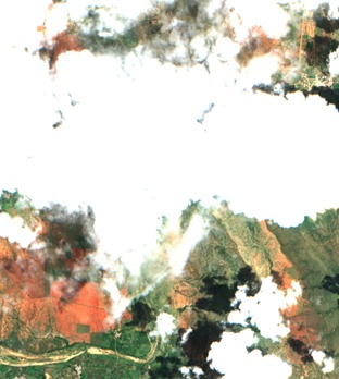
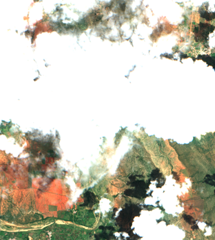
Example of a cloud obstructed view


Inspiration
Water availability is quite an essential factor for various purposes such as agriculture, domestic usage, industrial usage, etc. In the last few years, due to climate change, the regular weather patterns have been disrupted which in turn has affected water availability. The issue of water availability is extremely relevant in the Indian context, which is home to 18 percent of the world’s population, but possess only 4 percent of its water resources Ref. Studies show that 40% of the population will have absolutely no access to drinking water by 2030 Ref.
One of the major reasons for such a dire situation is the unplanned usage of water resources. One recent report mentions that nationally over 70% of the surface irrigation water is being simply wasted Ref. Besides the rate of groundwater extraction is also quite alarming. Water management, therefore, is the only way to treat India’s water crisis that will soon snowball into a national calamity.
So, in order to address these issues, sustainable usage of water resources is necessary. This can arise only from informed consumption. This is quite a challenge as there is not much awareness in the ground level about water usage planning. Only an informed consumer can be an empowered consumer. The planned and informed use of water can assist several sustainable development goals.
- Clean Water and Sanitation: To improve the standard of living and prevent many water-borne ailments which can lead to Good Health and Well-being
- Sustainable Cities and Communities: Can help authorities prevent periods of water stress and allocation between various sectors which can help in Responsible Consumption and Production
- Climate Action: The impact of climate change can be mitigated Industry, Innovation, and Infrastructure
If we can equip the communities at the ground level with the knowledge of water availability, this can empower them to make informed decisions for water usage planning. For example, depending upon the amount of water available, a farmer can decide what kind of seed to go with; the local authorities can decide on the actions required to be taken in case of water stress. This has a further advantage of addressing overuse of groundwater, which is a challenge in India. For this purpose, we want to make it possible for common people to monitoring local reservoirs and dams more accessible and easily understandable.
What it does
Our aim is to provide easy access to the climate trends to the commonest people. Hence, we prefer to provide the visual information to the end-user. Once the region is chosen, our analysis provides:
- Historical trends during summer
- The occasions of maximum and minimum moisture content
- Probable behaviour during peak summer once we have data from October to January/February
- Most probable state of the reservoir by visual information by referring to the historical data
How we built it
For this purpose, we use Sentinel 2 satellites L2A data. Sentinel-2 carries the Multispectral Imager (MSI). This sensor delivers 13 spectral bands ranging from 10 to 60-meter pixel size in visible spectrum, near infrared and short-wave infrared. Its blue (B2), green (B3), red (B4), and near-infrared (B8) channels have a 10-meter resolution. Next, its red edge (B5), near-infrared NIR (B6, B7, and B8A), and short-wave infrared SWIR (B11 and B12) have a ground sampling distance of 20 meters. Finally, its coastal aerosol (B1) and cirrus band (B10) have a 60-meter pixel size. It also provides AI-processed pixelwise classification data into water, soil, vegetation, snow, etc.
To measure the water content, one of the measures used is Normalized Difference Moisture Index (NDMI). It detects moisture levels in vegetation. It is calculated as a ratio between the NIR (Band 8A) and SWIR (Band 11) values of the satellite bands. The expression for calculating NDMI is:
NDMI = (B8A – B11)/(B8A + B11)
The maximum value possible for NDMI is 1 (corresponding to a water-logged area) and the minimum value possible is -1 (corresponding to a dry area). We considered using Normalized Difference Water Index (NDWI) which allows us to detect changes in water content of the water bodies. However, NDWI detects water content in clouds as well which leads to major fluctuations. On the other hand NDMI is neutral towards clouds, which doesn't create any major fluctuations in the measurement.
Challenges we ran into
However, the data from these different bands are not as clean as we would like it to be. Many a times, clouds affect the measurement. For example, if a cloud comes over a particular water body it can lead to the NDMI value being affected due to the water content in it. So, we must omit all the data where a lot of clouds are present. This is specifically challenging during the months of June-December when India experiences two seasons of monsoons.
- South-West Monsoon: June to September
- North-East Monsoon: October to December
The presence of clouds is extremely high specifically during the South-West monsoon. As a result, quite often none of the images taken during this period end up as useful. North-East monsoon exhibits this behaviour to a lesser extent. Thus, we may still get some data points during this period. In the months January-May, the obstruction due to clouds are far less. Hence, we need to exclude all those measurements when clouds obstruct the ground surface.
For this purpose, we used the neural networks-processed scene classification data obtained from the repository. This data tells us which of the pixels are probably clouds, vegetation, snow, etc. Ref. Though not 100% accurate, this information gives us a good estimate. With the help of this information, we excluded all the images with more than 20% of the pixels are defined as one form of cloud or another.
Since we are interested to monitor how a given water body changes its water levels during summer, this is all the information we need. Provided the coordinates of a waterbody, we can get the corresponding satellite data from the repository. It is to be noted that to get a better analysis, we need good data. Hence when providing the spatial coordinates of the lake, one must consider the maximum spatial extent to which the water body can spread out. One must also note that the assessment cannot be performed for small waterbodies like ponds or wells due to the limits in the resolution which is 20m per pixel. It is advised to consider waterbodies with dimension in km ranges.
What we learned
Once the NDMI values are obtained, we sum them for the selected region. It represents the water content available for the whole area in and around the water body. We then visualized and analysed how the NDMI sum for a region changes with time. It was observed that observed that the number of pixels with high NDMI values tend to decrease linearly from October to June. With the help of this, we can compare how much water is present initially in the reservoir and how fast it decreases every year. For example, a high value NDMI sum indicates abundance of water, which indicates that there might not be water stress during the summer. However, a faster decay of the NDMI sum indicates probable water stress. Based on this linear relation we can predict the water levels in the months leading up to the monsoon with a decent accuracy.
Next, let us consider the reservoirs that we used for our case study.
Case Study: Malavi Dam, Karnataka
Malavi reservoir was built in 1972 to augment rainwater and provide irrigation cover to few chronically drought-prone villages in the vicinity.
On comparison, we can see that the figure of Malavi dam on 27 May 2017 has just a few patches where NDMI value is high whereas the figure of Malavi dam on 29 Oct 2017 there is an abundance of moisture around.
In order to analyse the trends in moisture content, we used the sum of NDMI. That way we felt that it can account for the moisture content around the waterbody as well. The NDMI sum starts with a peak value for the year and reduces as the summer proceeds. One can also see that by end of February/beginning of March, the trend for the rest of the summer is set. For example, we can see that 2019 was one of the driest summers. Comparing 2022 and 2018, we can see that though the initial moisture content in January (0-30) was not the same, they ended up having similar NDMI by the end of May (~120). We can say that this is due to higher intensity of 2022 summer (though good rain was received in the latter half of 2021) as opposed to 2018.
So, once we have the data from October to January/February, we can predict what will be the NDMI sum for the region. Based on that value, we can find the point from historical data which will show the closest behaviour. This would help the people visualize how the summer will be.
Case Study: Gandipalem, Andhra Pradesh
Gandipalem Project was constructed during period of 1975 to 1984 about across Pillaperu river. The dam was built as the irrigation source for 17 villages located in drought areas in Udaygiri and Varikuntapadu Mandals. The irrigated area registered under the project is 10.26 km².
In order to analyse the trends in moisture content, we again used the sum of NDMI. One can also see that by end of February/beginning of March, the trend for the rest of the summer is set. For example, we can see that 2019 was one of the driest summers as in the case of Malavi dam. However, 2019 also was quite a dry year in this case. Comparing 2022 and 2020, we can see that though the initial moisture content in January (0-30) was similar, they ended up having different NDMI in March and April (~120). The behaviour of NDMI in this reservoir is not as straightforward as Malavi.
Nonetheless, the change in NDMI is more or less linear. What one should notice is that there is scant data during November and December. This place is closer to East Coast where North-West Monsoon is stronger in these months, hence this behaviour. So, once again, once we have the data from October to February, we can predict what will be the NDMI sum for the region. Based on that value, we can find the point from historical data which will show the closest behaviour. This would help the people visualize how the summer will be.
From these two case studies, we can see that it’s better to have data up to at least February or March to predict the trend for the summer.
What's next for Waterbody monitoring
With this solution what we seek to do is to empower the people at the ground level who are not necessarily tech savvy. We would like to provide them a visual information how the waterbody would look on a given date in the summer. With enough enough data from Sentinel 2 repository, we can recall any of the historical data to make the end user to empower the end user. With this we seek to bring benefits of ML to the commonest of the people.
The current algorithm is aimed at places in the Indian subcontinent where the impact of monsoons in pronounced. However, there are other climatic zones which are not necessarily influenced by monsoons as much such as deserts, Himalayan mountains etc. We would like to undertake a better study of these regions and examine the possible similar solutions.
Built With
- jupyter
- python
- satsearch
- sentinel
- sklearn


Log in or sign up for Devpost to join the conversation.