-
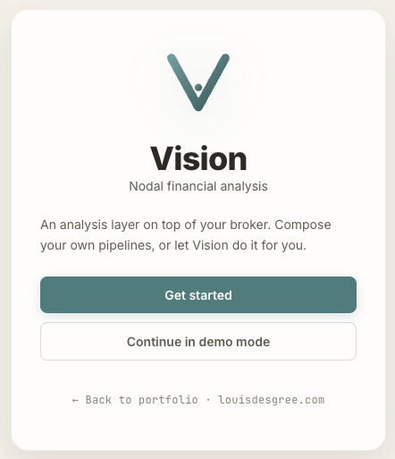
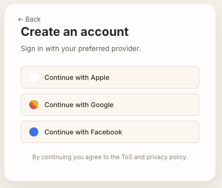
User Entry point
-
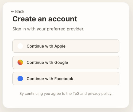
Authentication
-

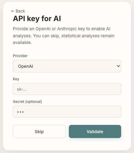
Allow the user to connect with his API key to enable deeper analysis
-
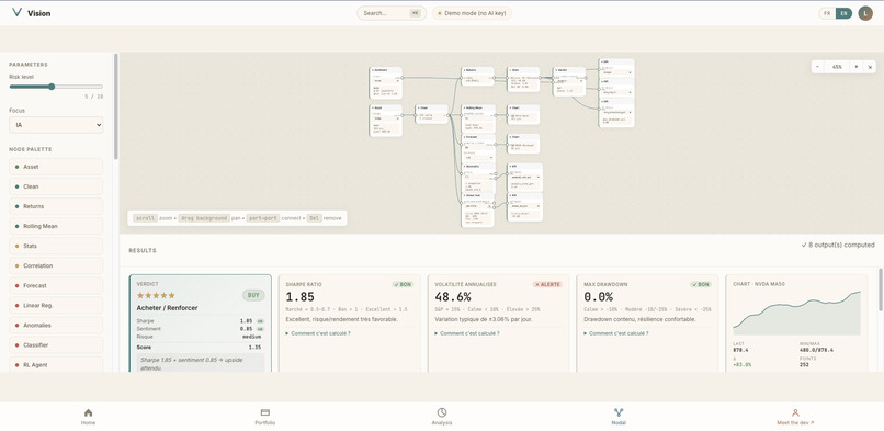
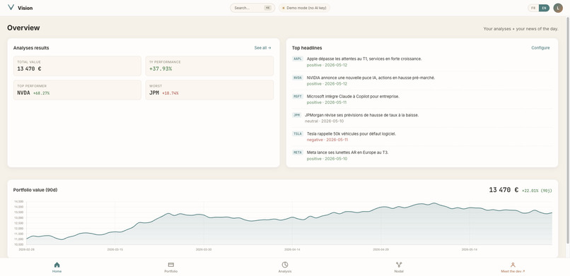
Nodal interface enabeling the user to run his own analysis
-
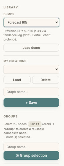
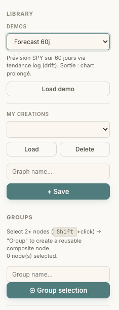
In the user interface the user can load premade demos and group his nodes into a single node allowing more complex procedures
-
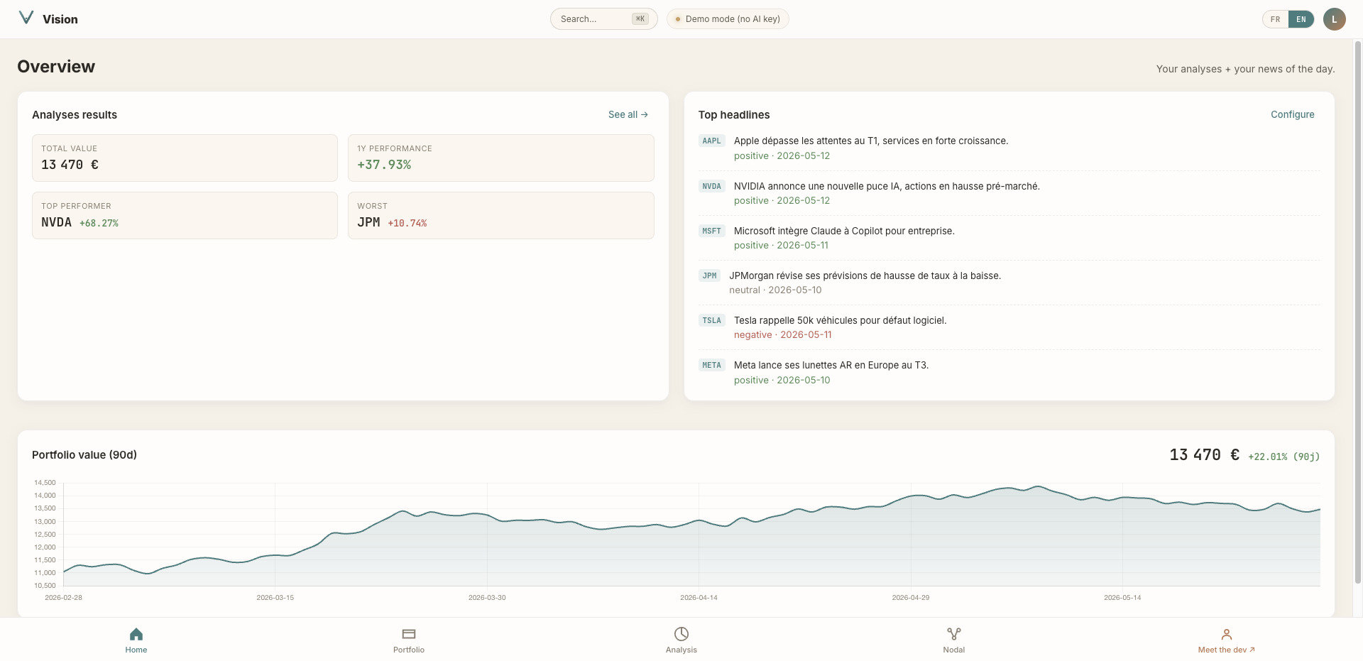
Home page showing markets trends and user main kpi's
-
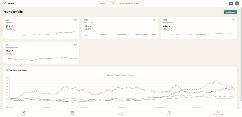
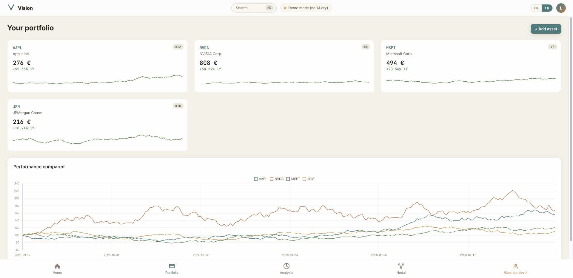
User Portolio page
-
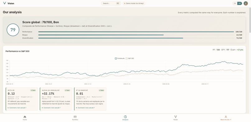
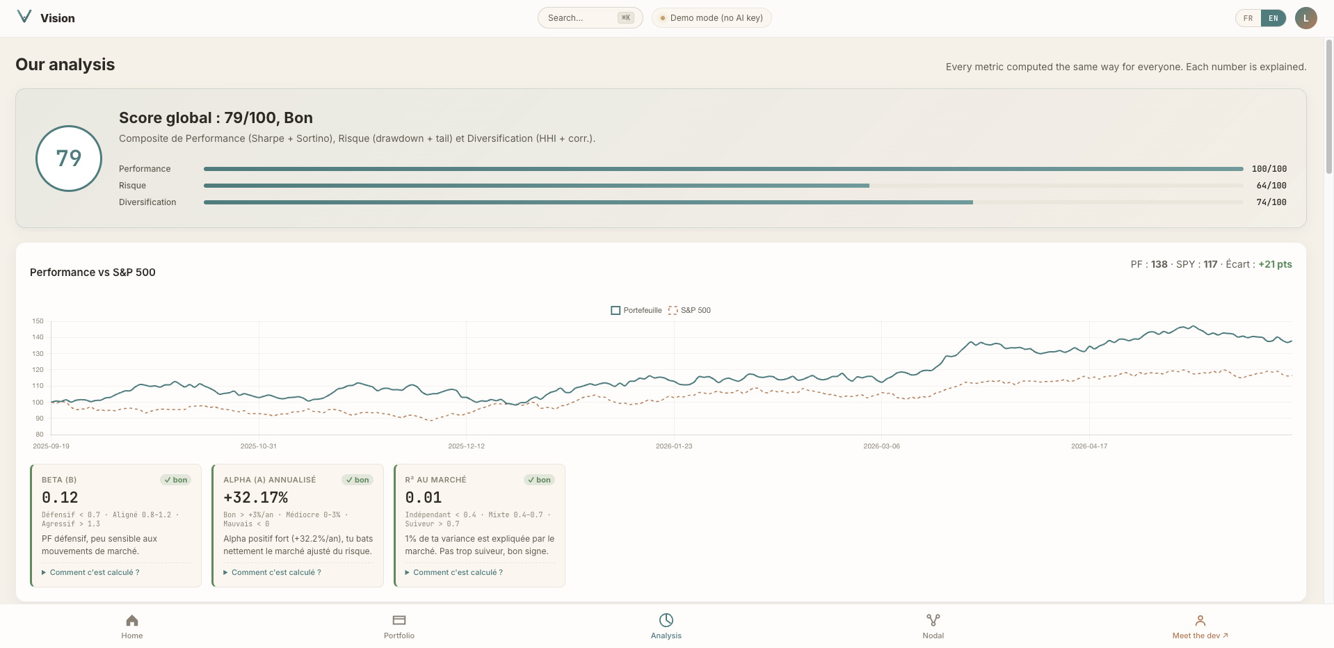
Autonomous analysis of the user portfolio
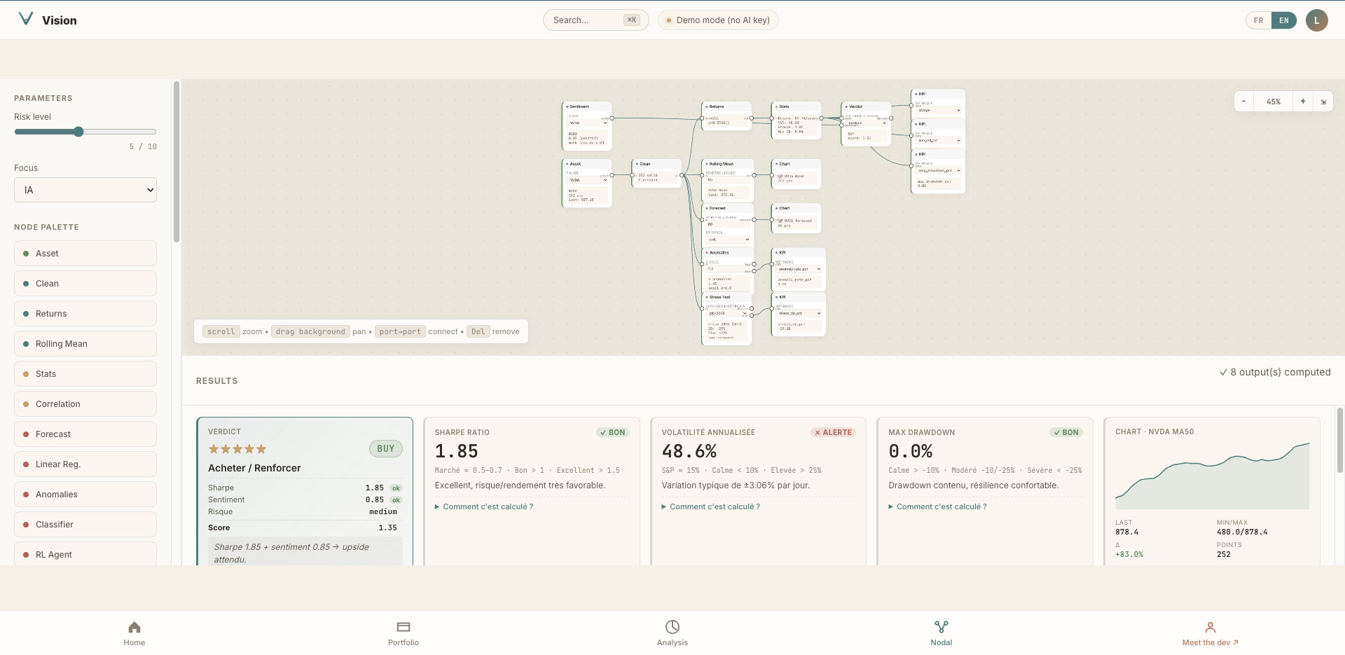
Vision
A composable, pedagogical, anti-Bloomberg portfolio analysis tool. Built for the curious investor who wants to understand, not to be told what to buy.
Inspiration
I love finance, but building a portfolio is hard. The information you get is filtered by your broker. Pre-chewed cards, opaque "AI insights", and zero composability. If you want to actually understand your portfolio, measure its tail risk, simulate what a 2008-style crash would do to it, see how political news might shift sentiment, you're stuck between dumbed-down retail feeds and a \$25k/year Bloomberg terminal.
I built Vision to fill that gap. The philosophy is simple. Don't tell people what to buy. Let them do data science on their own portfolio. Let them cross it with media and politics. Let them plug in a bit of machine learning. Let them walk out understanding why a number means what it means.
The big idea, a nodal canvas for finance
Instead of fixed dashboards, Vision is a composable node graph. Think Touch Designer or Houdini, but for portfolio analysis. Every connection is type checked. The graph runs in real time, client side.
A minimal verdict pipeline:
 ┌───────┐  prices  ┌───────┐   out   ┌─────────┐   out   ┌───────┐  stats  ┌─────────┐
 │ Asset │ ───────► │ Clean │ ──────► │ Returns │ ──────► │ Stats │ ──────► │ Verdict │
 └───────┘          └───────┘         └─────────┘         └───────┘         └─────────┘
Fork the same Clean output across five parallel branches and you get a full quant lab on one screen:
                                  ┌──► Returns ───► Stats ───► Verdict
                                  │
                                  ├──► RollingMean ──► Chart  (moving average)
   ┌───────┐         ┌───────┐    │
   │ Asset │ ──────► │ Clean │ ───┼──► Forecast ─────► Chart  (60 day projection)
   └───────┘         └───────┘    │
                                  ├──► Anomalies ────► KPI    (z score outliers)
                                  │
                                  └──► StressTest ───► KPI    (GFC 2008)
The current build ships 23 node types across 6 categories (source, transform, analysis, ML, output, group) and 14 pre built demos showing how they compose.
How the engine works
Every change triggers a topological sort then a single evaluation pass:
G = (V, E)                  V = nodes, E = typed edges
order = TopoSort(G)
for each node n in order:
    inputs  = read outputs of upstream connected nodes
    outputs = n.compute(inputs, params)
Type checking lives on the edges. A series cannot plug into a stats input. The error fires the moment you drop the wire, not at runtime. A debounced autosave persists the full graph to localStorage on every change.
The metrics, with intuition first
This is where the pedagogy lives. Each metric on the Auto Analysis page comes with a benchmark range, a plain English interpretation, and a How is this computed? toggle. Sharpe alone misses everything that matters about tail risk. Here is the honest set.
Return per unit of risk
Sharpe ratio answers am I rewarded enough for the risk I take?
              annualized return
Sharpe  =  ───────────────────────
             annualized volatility
The S&P 500 sits around 0.5 to 0.7 long term. Above 1 is good. Above 1.5 is excellent.
Sortino ratio is Sharpe's smarter cousin. It only penalizes bad volatility (the days you lose), not the days you gain.
                 annualized return                 1
Sortino  =  ─────────────────────────   ,   σ²  = ─── × Σ rᵢ²   (only rᵢ < 0)
                  σ_downside              down     N
A portfolio with a Sortino much higher than its Sharpe has asymmetric volatility (more upside spikes than downside).
Calmar ratio compares your return to your worst historical drawdown. It answers how much pain did I have to endure for this return?
              annualized return
Calmar  =  ───────────────────────
              | Max Drawdown |
Above 1 means you earn more per year than your worst crash cost. Above 3 is hedge fund grade.
Tail risk
Value at Risk (VaR) is the daily loss you will exceed only 5 days out of 100.
VaR₉₅ = 5th percentile of daily returns
Critical caveat. VaR says nothing about how bad the worst 5% actually is. So we also compute CVaR (Expected Shortfall), the average loss given that you are in the worst 5%.
CVaR₉₅ = E[ r | r ≤ VaR₉₅ ] average of the worst 5% of days
Basel III mandates CVaR specifically because VaR alone hides the fat tails.
Distribution shape
Skewness measures whether your returns lean toward gains or toward losses.
              E[ (r − μ)³ ]
Skew  =  ──────────────────────
                  σ³
Negative skew means more crashes than rallies. Most equities sit at slightly negative skew.
Excess kurtosis measures how thick the tails are.
                  E[ (r − μ)⁴ ]
K_excess  =  ──────────────────────   −  3
                       σ⁴
A Gaussian distribution scores 0. Real markets routinely score above 3. That extra mass in the tails is exactly where black swans live, and where Gaussian models lie to you.
Market exposure (CAPM)
Beta is how much your portfolio amplifies the market.
            Cov(R_a, R_m)
β  =  ────────────────────────
              Var(R_m)
A beta of 1.5 means when the S&P moves 1%, you move 1.5% on average. Beta below 0.7 is defensive (utilities, staples). Beta above 1.3 is aggressive (small caps, tech).
Jensen's alpha is the return you generate beyond what your beta predicts. It is the purest measure of stock picking.
α = ( R̄_a − β × R̄_m ) × 252
Positive alpha means you beat the market at equal risk. Most active managers post negative alpha over the long run.
Diversification
The Herfindahl Hirschman Index measures concentration. Sum of squared weights.
              n
HHI  =       Σ      wᵢ²
             i=1
A perfectly equal weighted portfolio of N assets has HHI = 1/N. A portfolio entirely in one asset has HHI = 1. Above 0.25 is concentrated.
From HHI we derive the effective number of bets.
              1
N_eff  =  ───────
             HHI
You may hold 10 positions but if 80% sits in one of them, your N_eff is closer to 1.5 than 10.
The average pairwise correlation tells you whether your assets actually move independently.
              1
ρ̄  =  ─────────── ×  Σ    ρ(i, j)
          C(n, 2)     i<j
If ρ̄ > 0.7 your diversification is cosmetic. You are really holding one bet.
Risk attribution
A position can be 25% of your value but contribute 40% of your risk. The two donuts side by side reveal it instantly. Formally, the percentage contribution to risk.
              wᵢ × Σⱼ wⱼ × Cov(i, j)
PCR(i)  =  ─────────────────────────         and       Σᵢ PCR(i) = 1
                      σ_p²
This is the metric most retail apps refuse to show because it is the one that exposes hidden concentration.
Stress tests, the same asset under 4 historical regimes
The StressTest node projects how your asset would behave under a calibrated historical crisis. Each scenario is a deterministic Gaussian random walk.
v(t+1) = v(t) × ( 1 + μ_s + σ_s × z_t ) z_t ∼ N(0, 1)
The drift μ_s and volatility σ_s are calibrated on real history.
| Scenario | μ_s per day | σ_s | Duration | Expected loss |
|---|---|---|---|---|
| GFC 2008 | −0.52% | 1.6% | 130 days | ≈ −49% |
| COVID 2020 | −1.25% | 2.8% | 33 days | ≈ −34% |
| Rates 2022 | −0.115% | 1.2% | 250 days | ≈ −25% |
| Dotcom 2000 | −0.30% | 2.0% | 500 days | ≈ −78% |
The RNG seed comes from the scenario name. Same scenario, same trajectory, every time.
Political scenarios, what if quantified
Same machinery, applied to forward looking events. Pick a scenario, get a stressed path.
                            ┌──────────────────────────┐
                            │  Tariffs USA China 25%   │
   ┌───────┐   ┌───────┐    │   μ = −0.30%/d           │   ┌─────────┐
   │ Asset │──►│ Clean │ ──►│   σ =  1.80%/d           │──►│ Chart   │
   └───────┘   └───────┘    │   T = 60 days            │   └─────────┘
                            └──────────────────────────┘
Seven calibrated scenarios. Tariffs USA China. Banking crisis. Strict AI regulation. Energy shock. Pro business electoral surprise. Geopolitical conflict. Dovish Fed pivot.
News integration, narrative becomes signal
Headlines turn into a tractable input to the verdict graph.
 ┌─────────┐  news   ┌────────────┐  news   ┌────────────────┐  sentiment   ┌─────────┐
 │NewsFeed │ ──────► │ NewsFilter │ ──────► │ NewsSentiment  │ ───────────► │ Verdict │
 └─────────┘         └────────────┘         └────────────────┘              └─────────┘
                            │
                            └─► Headlines (display)
Each news item carries a sentiment score s_i in [−1, +1] and an editorial relevance r_i in [0, 1]. The aggregator is a relevance weighted mean.
              Σᵢ ( sᵢ × rᵢ )
S_news  =  ────────────────────
                  Σᵢ rᵢ
For recency weighting, the weight decays with age.
                    1
wᵢ   ∝   ─────────────────────
            √ ( t_now − tᵢ )
The EventImpact node then projects this aggregated sentiment forward as a drift on the price series.
μ_news = 0.0015 × S_news × magnitude
A daily drift of 0.15% over 30 days compounds to roughly +4.5% (or −4.5%) on top of the current price. Small per day, real per month.
Composite nodes, grouping is a first class operation
Select N nodes, hit Group. Vision auto detects the external interface, collapses the selection, and registers the result as a brand new node type in the palette.
Before                                       After

 ┌─────┐  ┌─────┐  ┌────────┐                 ┌──────────────────┐
 │Asset│─►│Clean│─►│Returns │                 │ Prepared Returns │
 └─────┘  └─────┘  └────────┘                 │ param: ticker    │
                                              │ out:   returns   │
                                              └──────────────────┘
The detection rules are pure set theory. Let S be the selected nodes.
Inputs(S)   =  { e ∈ E  |  target(e) ∈ S   ∧   source(e) ∉ S }

Outputs(S)  =  { (n, p)  |  n ∈ S   ∧   ( used externally  ∨  unused internally ) }
An input of the group is any edge whose target lives in S but whose source does not. An output port is any inner port that either feeds something outside the group, or feeds nothing internally (so the user can wire it later). Inner edges and inner parameters stay inside. The group is persisted to localStorage so it survives reloads.
What you can do
- Backtest 4 strategies (momentum, mean revert, trend, AR(1)) against buy and hold in one click.
- Stress test the same asset across 4 historical regimes simultaneously.
- Project political scenarios. What happens to NVDA if US China tariffs escalate?
- Aggregate real news into a weighted sentiment that feeds your verdict.
- Compose your own nodes from any selection.
- Save and share graphs (autosave, named saves, composite types).
- Command palette (⌘K) for navigation, search, and every action.
- Toggle EN / FR on every screen, persisted across sessions.
How I built it
Pure vanilla web. No framework. No build step. Single index.html, styles.css, data.js, canvas.js, app.js, lang.js. Chart.js loaded from CDN.
Mock financial data is generated client side via seeded Box Muller random walks. Geometric Brownian motion calibrated per ticker.
r_t = μ + σ × √ ( −2 × ln u₁ ) × cos ( 2π × u₂ ) u₁, u₂ ∼ U(0, 1)
The canvas is hand built. SVG bezier wires. World↔screen coordinate transforms for pan and cursor anchored wheel zoom. Type checked port connections. Debounced autosave. Composite node compilation. Command palette over every action.
Challenges
Cursor anchored zoom in a transformed viewport. Innocent looking until you implement it. The world point under the cursor must stay fixed in screen space across a scale change. Three lines, but the order matters.
1. read cursor position in world coords:
   (xw, yw)  =  ( (xs − px) / z ,  (ys − py) / z )

2. apply zoom:
   z  ←  z × 1.12

3. re-anchor pan so the world point stays under the cursor:
   (px, py)  =  ( xs − xw × z ,  ys − yw × z )
SVG paths need vector-effect: non-scaling-stroke to stop looking weird at 200% zoom.
Composite nodes. Auto detecting the external interface from an arbitrary selection took roughly 400 lines. Inner subgraph execution runs in isolation at compute time, with external inputs pre fed and exposed outputs collected.
A type system that scales without being bureaucratic. Started with strict types (series, returns, stats, news, sentiment, scalar all distinct). Hit "you can't connect Returns to Stats" instantly. Iterated until types are meaningful but not in the way. The Stats node accepts a generic series input and internally detects whether it is looking at prices or returns.
Designing 23 nodes that compose meaningfully. Each node must produce outputs that some other node actually consumes. Took several rewrites. The EventImpact node separates the news input from the price input so each can be tweaked independently.
Auto narrative without sounding like a robot. The Insights paragraph reads like a senior advisor. Specific numbers. Names both strengths and weaknesses. Closes with an action oriented line. Generated by conditional logic over the metric grid.
Full EN / FR coverage on a vanilla web stack. No i18n library. A 60 line lang.js exposes t(en, fr) and walks data-i18n-en / data-i18n-fr attributes. Every dynamic structure (KPI registry, demo catalog, glossary) stores {en, fr} objects resolved at render time. Lang toggle triggers a full re render of the canvas so node param labels switch live.
What I learned
- Finance metrics are deeper than they look. Sharpe alone misses everything that matters about tail risk. Sortino, Calmar, CVaR, skewness, and excess kurtosis form the honest set.
- The hardest part of a finance UI is not the math. It is the teaching. Every number needs a benchmark, an interpretation, and a formula on demand.
- News and politics can be quantified into a pipeline. Headlines become a weighted scalar. The scalar drives a verdict. Soft becomes hard.
- Composability beats configurability. 23 small bricks beat 50 toggles on a fixed dashboard.
Vision is the finance tool I wanted when I started investing and could not find. Now it exists.
Built With
- anthropic
- capm
- chart.js
- claude-ai
- css3
- data-science
- finance
- geometric-brownian-motion
- github
- github-actions
- html5
- javascript
- localstorage
- machine-learning
- mathjax
- neuralprophet
- openai
- portfolio-theory
- python
- scikit-learn
- statsmodels
- svg
- yfinance

Log in or sign up for Devpost to join the conversation.