-
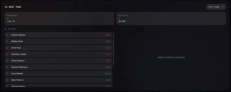
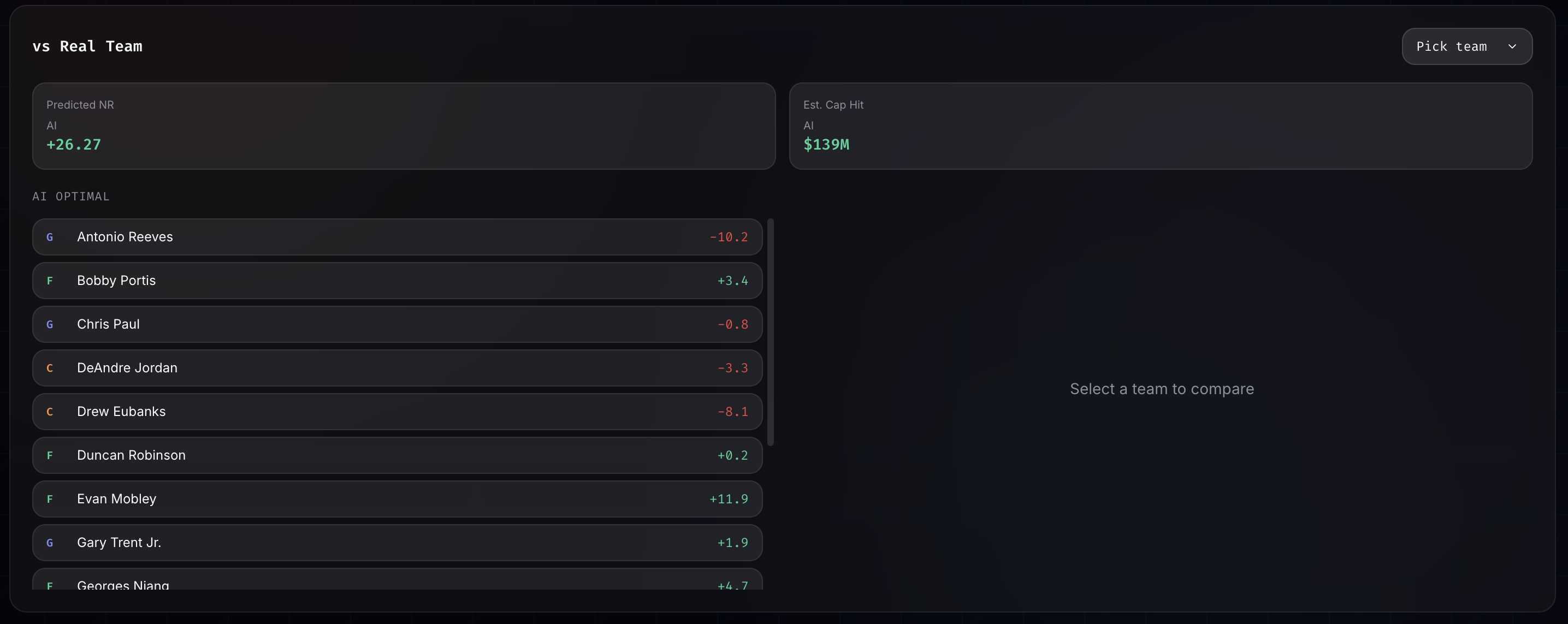
Lineup comparison tool for comparing across existing rosters in NBA
-
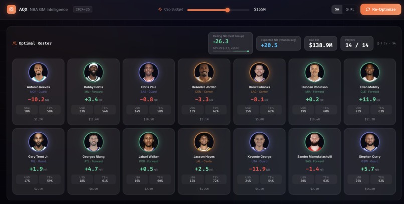
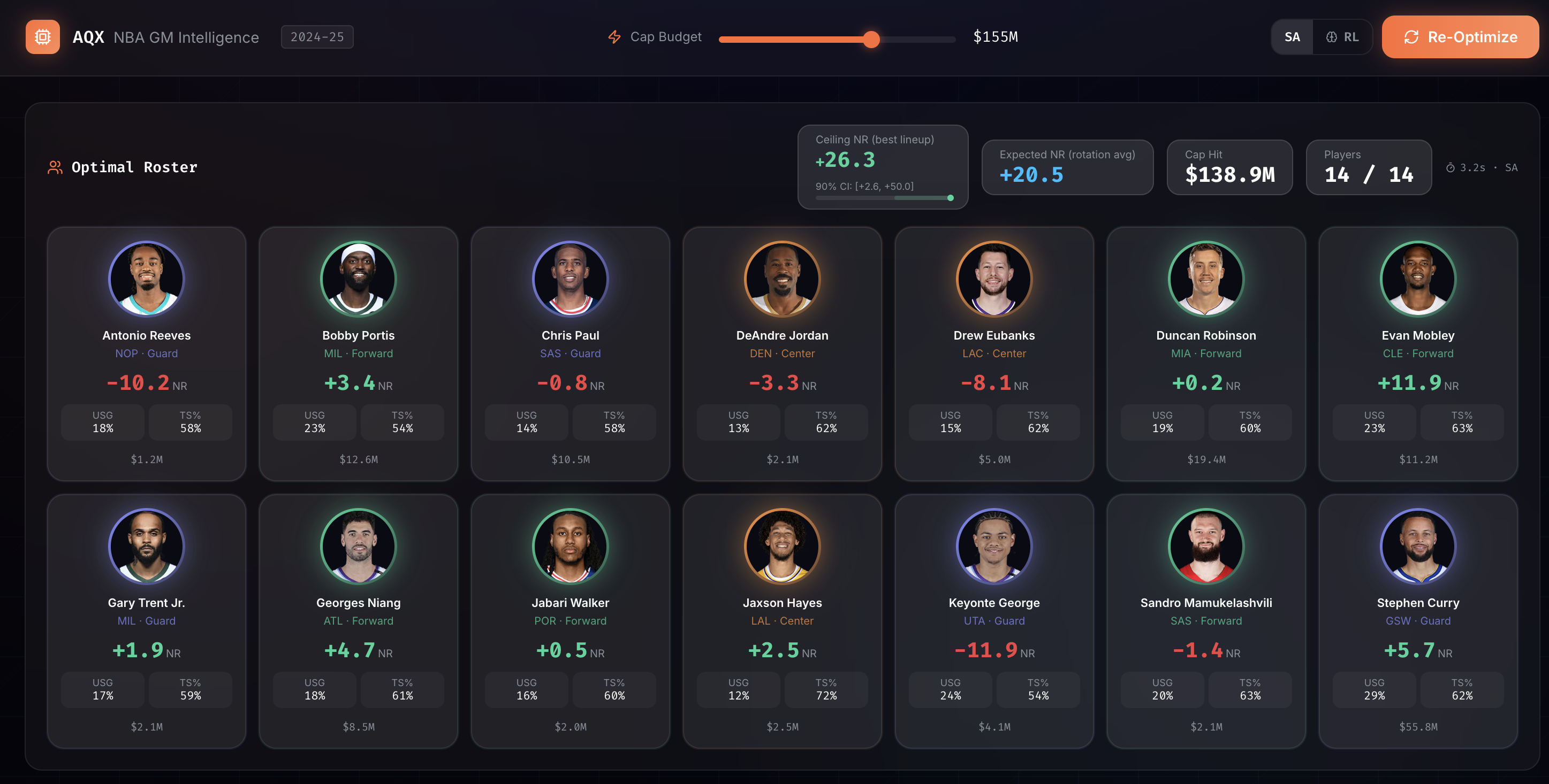
Optimal Roster Screenshot
-
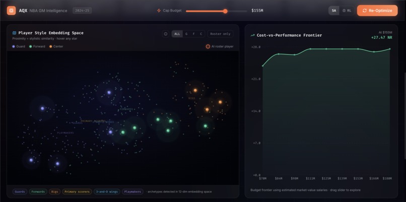
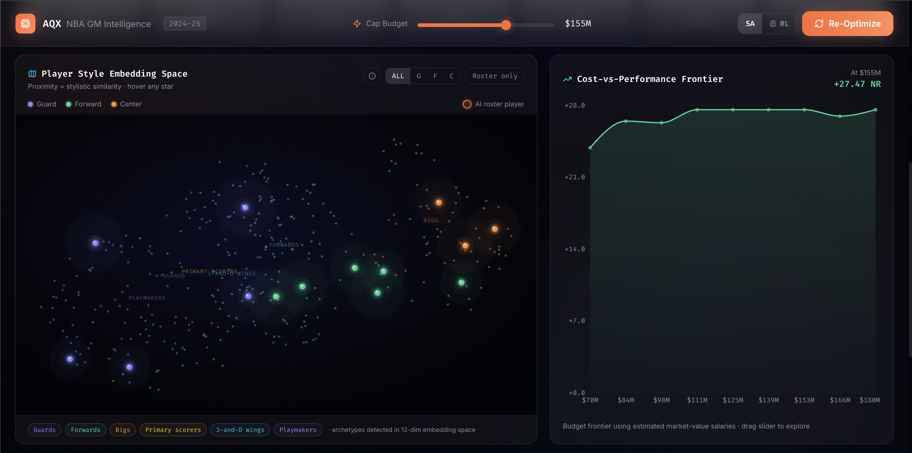
Visualisations to show relative effect of roster compared to Cost
Inspiration
What it does
How we built it
Challenges we ran into
Accomplishments that we're proud of
What we learned
What's next for Virtual_NBA_GM
1. About the Project
Inspiration
The idea started with a simple observation: every public "roster optimiser" tool reduces players to a single number and adds them up. A team of five 30-point scorers does not produce 150 points a game. There is one ball, roughly 100 possessions, and what actually determines how a lineup performs is not the sum of its parts — it is how those parts interact with each other.
At the same time, the problem maps almost exactly onto something I find genuinely interesting in quantitative finance. A general manager assembles a portfolio of players under a budget (the salary cap), where each asset has an expected return (how much they raise the team's point differential) and a price (their cap hit). The cap is the budget constraint. Roster construction is portfolio selection.
That double insight — that player identity needs a richer representation than a scalar, and that lineup performance is non-additive — became the architectural spine of the entire project.
How I Built It
The system is a four-stage ML pipeline, each stage with a clean interface to the next.
Stage 1 — Player Embeddings
Each player-season is described by 19 per-100-possession and rate statistics. These are z-scored using a scaler fitted on training seasons only (2014–22), then passed through a denoising autoencoder that compresses them into a 12-dimensional bottleneck:
$$ \mathcal{L}{\text{recon}} = \frac{1}{N} \sum{i=1}^{N} \left| \hat{x}_i - x_i \right|^2 $$
where $\hat{x}_i = \text{Decoder}(\text{Encoder}(x_i + \epsilon))$ and $\epsilon \sim \mathcal{N}(0, \sigma^2)$ is injected noise. A PCA baseline is fit at the same dimensionality for comparison.
To push the embeddings beyond individual identity and toward co-performance, I added a synergy contrastive loss. For every qualifying training lineup, all $\binom{5}{2} = 10$ player pairs are extracted and labelled with a similarity target derived from the lineup's net rating:
$$ \text{target}{(a,b)} = \tanh!\left(\frac{\text{NR}{\ell}}{12}\right) $$
The contrastive loss is a possession-weighted MSE between the actual cosine similarity of the two embeddings and this target:
$$ \mathcal{L}{\text{contr}} = \sum{\text{pairs}} w_{(a,b)} \cdot \left(\cos(z_a, z_b) - \text{target}_{(a,b)}\right)^2 $$
where $w_{(a,b)} = \log(1 + \text{POSS}_\ell)$. The combined objective is:
$$ \mathcal{L} = \mathcal{L}{\text{recon}} + 0.25 \cdot \mathcal{L}{\text{contr}} $$
This produced 27,020 co-performance pairs from 2,722 training lineups. Post-training, the correlation between embedding cosine similarity and the NR target reached +0.31, confirming the embeddings absorbed synergy signal. A UMAP projection of the 12-dimensional space clusters guards, forwards, and centers naturally — without position labels being supplied during training.
Stage 2 — RAPM and the Lineup Fit Model
Raw lineup net rating is confounded. A lineup looks good partly because of the players' individual quality and partly because of fit and interaction effects. Training a model to predict raw NR mixes these two signals, and because individual quality dominates, interaction models gain nothing over a simple mean-pool of embeddings.
The fix is Lineup-Adjusted Plus-Minus (RAPM proxy): for every player $i$, estimate their individual contribution $\beta_i$ by solving a possession-weighted ridge regression over all training lineups:
$$ \hat{\beta} = \arg\min_\beta \sum_\ell w_\ell \left( \sum_{i \in \ell} \beta_i - \text{NR}_\ell \right)^2 + \lambda |\beta|^2 $$
where $w_\ell = \log(1 + \text{POSS}_\ell)$ and $\lambda = 100$ (chosen by 5-fold cross-validation). This explains 24.5% of lineup NR variance on the training set. The residual is the interaction effect the fit model targets:
$$ \text{RAPM_RESIDUAL}\ell = \text{NR}\ell - \sum_{i \in \ell} \hat{\beta}_i $$
The fit model — a Set Transformer (pre-norm TransformerEncoder, $d=64$, 4 heads, 3 layers, no positional encoding) — is trained to predict this residual from the five players' embeddings. Permutation invariance is guaranteed by design: no positional encoding is added, and the readout is mean-pool over the five output tokens. The training loss is possession-weighted MSE on the residuals:
$$ \mathcal{L}{\text{fit}} = \sum\ell \frac{\text{POSS}\ell}{\sum\ell \text{POSS}\ell} \cdot \left(\hat{r}\ell - \text{RAPM_RESIDUAL}_\ell \right)^2 $$
The model is trained on seasons 2014–22 and validated on 2022–25 — a strict season-based split that prevents any future lineup information from entering training. The full prediction at inference time is:
$$ \widehat{\text{NR}}\ell = \underbrace{\sum{i \in \ell} \hat{\beta}i}{\text{individual quality}} + \underbrace{\hat{r}\ell}{\text{interaction effect}} $$
A six-model ablation (mean-pool, GATConv GNN, Transformer $\times$ PCA/AE embeddings) showed that with RAPM-residual targets, the Transformer/AE configuration achieves best wMAE of 8.63 — its first win over mean-pool. This is the scientific result of the project: removing the additive individual-quality component surfaces the interaction signal that multi-head attention is genuinely suited to model.
Conformal prediction intervals are derived from the 903-lineup validation set. Using split conformal calibration:
$$ q_{90} = \text{Quantile}{90\%}!\left( \left{ \left|\hat{r}\ell - r_\ell\right| \right}{\ell \in \mathcal{D}{\text{cal}}} \right) = \pm 23.7 \text{ NR points} $$
This gives a finite-sample guarantee: the 90% prediction interval $[\widehat{\text{NR}} - q_{90},\ \widehat{\text{NR}} + q_{90}]$ contains the true lineup NR with at least 90% probability under exchangeability, without any distributional assumption on the residuals.
Stage 3 — Roster Optimizer
A roster's score is defined as the maximum predicted NR over all $\binom{8}{5} = 56$ five-man lineups drawn from the top-8 rotation players (sorted by GP):
$$ \text{score}(R) = \max_{\ell \subseteq \text{top8}(R),\,|\ell|=5} \widehat{\text{NR}}_\ell $$
Three search strategies are implemented:
Simulated annealing with $T_0 = 5.0$ and geometric cooling rate $\alpha = 0.9975$, run for 10,000 iterations over 3 restarts. At each step a random swap is proposed and accepted with probability $\min(1,\, e^{\Delta s / T})$.
Genetic algorithm with population 150, 300 generations, set-union crossover, and tournament selection ($k=5$), enforcing feasibility via a penalty:
$$ \text{fitness}(R) = \text{score}(R) - 8 \cdot \text{pos_violations}(R) - 50 \cdot \max!\left(0,\, \frac{\text{salary}(R) - C}{10^6}\right) $$
REINFORCE policy-gradient agent trained over 20,000 episodes. The state is the concatenation of 14 roster player embeddings (168-dim) with budget and position fractions (4-dim). The policy $\pi_\theta(a | s)$ selects which of the 14 slots to swap:
$$ \nabla_\theta J(\theta) = \mathbb{E}\pi \left[ \sum{t=0}^{T} \nabla_\theta \log \pi_\theta(a_t | s_t) \cdot \hat{A}_t \right] $$
where $\hat{A}t = G_t - V\phi(s_t)$ is the advantage with value baseline $V_\phi$, and an entropy bonus $H(\pi_\theta)$ encourages exploration. After training the policy achieves inference in ~1 second versus simulated annealing's 3 seconds, with best predicted NR of +21.7.
Stage 4 — Dashboard
A FastAPI backend pre-computes the optimal roster, 9-point budget frontier, nearest-neighbour similarity index, and six player archetype cluster centroids on startup, caching everything to disk. A React frontend serves four panels: the 14-player roster grid with NBA CDN headshots; a custom SVG UMAP galaxy where roster players glow as animated multi-layer orbs connected by constellation lines to their nearest stylistic neighbours; a cost-vs-performance frontier area chart with a live budget reference line; and a real-team comparison panel across all 30 NBA franchises.
What I Learned
Honest results matter more than impressive ones. The GNN is architecturally correct for this problem. With 998 training lineups it overfit; mean-pool won. The right move was to report this honestly and explain why, rather than force a GNN result or hide the ablation. The RAPM decomposition then gave the Transformer the conditions it needed to finally outperform — and that story, where you explain why a fancier model wins under specific conditions, is far more credible than one that just claims it works.
Data engineering is the load-bearing wall. Stats.nba.com uses JA3/JA3S TLS fingerprint inspection to block non-browser clients. Discovering this took an afternoon; patching it with curl_cffi took ten minutes. The salary join had a similar profile — _fmt_season converting Year=2025 to "2024-25" is a one-liner that unlocks 89% salary coverage. Mundane problems eat the most time.
Fast inner loops are an architectural constraint, not an afterthought. The Transformer runs ~40× slower per evaluation than a 2-layer MLP. When I put it in the SA inner loop, 30,000 roster evaluations took over 60 seconds per call and broke the endpoint. The architecture has to separate the search model (fast, consistent relative rewards) from the final scorer (accurate, called once). Getting this wrong stalled the project for hours.
Conformal prediction is underused. A model that outputs "+13.6 NR" without uncertainty is giving a false impression of precision. The ±23.7 point 90% interval is wide — and that honesty is the point. A real front office should know the model is uncertain, not be misled by a number that implies it isn't.
Challenges
TLS fingerprinting on stats.nba.com. Standard Python requests gets silently dropped at the SSL layer. The NBA server completes the TLS handshake and then closes the connection without sending an HTTP response — exit code 56 from curl. The fix was curl_cffi, which impersonates Chrome's exact cipher suite order and extension set. Not obvious, not documented anywhere useful.
The GNN that wouldn't generalise. With 998 training lineups, the GATConv model peaked around epoch 50 and then overfitted monotonically while training loss kept falling. Every tuning attempt (learning rate, dropout, hidden dim, L2 weight) moved the peak epoch but didn't close the gap to mean-pool on wMAE. The only fix that actually worked was removing the dominant individual-quality signal via RAPM, which gave the interaction model a cleaner target. That took several iterations to understand.
Salary join edge cases. Kaggle salary data uses Basketball Reference conventions: Year=2025 means the 2024-25 season. Player names have accents, suffixes, and alternate spellings. The normalisation function (re.sub(r"[^a-z ]", "", name.lower())) plus the year conversion got coverage to 89% — the remaining 11% were handled with an NR-tier salary estimate so the optimizer couldn't treat unmatched stars as free agents. Getting Giannis and LeBron to cost $48M rather than $0 in the cap model was a necessary debugging step.
Making embeddings legible. The UMAP axes have no interpretable label. Telling a non-technical judge "proximity means similarity" is true but not compelling. The solution was: show the clustering (guards, forwards, centers separate naturally without labels), show the nearest neighbours in the tooltip (Curry → Lillard/Kyrie/Harden), and show the roster players glowing in different parts of the space. The visual does the explanation that words struggle to.
RL training time with the Transformer. The first attempt at re-training the RL agent after switching the ablation winner to the Transformer ran score_lineups() through the full attention mechanism in the inner batch loop — 40 candidates × 56 lineup combinations × full Transformer forward pass, repeated for every episode step. 20,000 episodes would have taken approximately 9 hours. The fix was a dedicated fast inner-loop model (MeanPoolBaseline) for the RL environment's reward signal, with the Transformer reserved for final evaluation. The architectural separation that was needed for SA was needed for RL as well.
Built With
- fastapi
- kaggle
- nba-api
- numpy
- pandas
- python
- pytorch
- react
- scikit-learn
- scipy
- typescript
- uvicorn

Log in or sign up for Devpost to join the conversation.