Using GCNs for Single-Cell Classification

• 

  Final Project Poster

Using Graph Convolutional Networks for Single-Cell Classification

Madeline Hughes (mhughe10), Nitya Thakkar (nthakka3)

Introduction

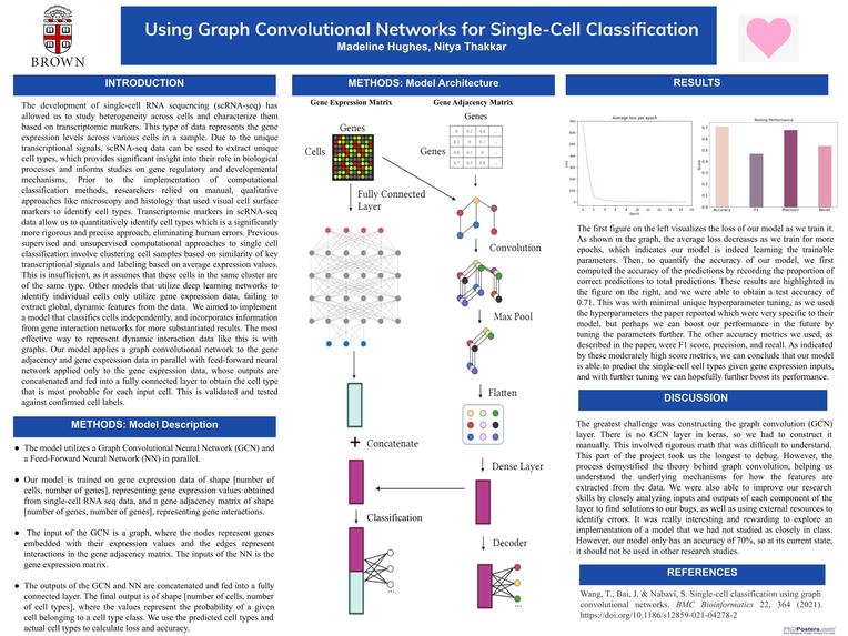
The development of single-cell RNA sequencing (scRNA-seq) has allowed us to study heterogeneity across cells and characterize them based on transcriptomic markers. This type of data represents the gene expression levels across various cells in a sample. Due to the unique transcriptional signals, scRNA-seq data can be used to extract unique cell types, which provides significant insight into their role in biological processes and informs studies on gene regulatory and developmental mechanisms. Prior to the implementation of computational classification methods, researchers relied on manual, qualitative approaches like microscopy and histology that used visual cell surface markers to identify cell types. Transcriptomic markers in scRNA-seq data allow us to quantitatively identify cell types which is a significantly more rigorous and precise approach, eliminating human errors. Previous supervised and unsupervised computational approaches to single cell classification involve clustering cell samples based on similarity of key transcriptional signals and labeling based on average expression values. This is insufficient, as it assumes that these cells in the same cluster are of the same type. Other models that utilize deep learning networks to identify individual cells only utilize gene expression data, failing to extract global, dynamic features from the data. We aimed to implement a model that classifies cells independently, and incorporates information from gene interaction networks for more substantiated results. The most effective way to represent dynamic interaction data like this is with graphs. Our model applies a graph convolutional network to the gene adjacency and gene expression data in parallel with feed-forward neural network applied only to the gene expression data, whose outputs are concatenated and fed into a fully connected layer to obtain the cell type that is most probable for each input cell. This is validated and tested against confirmed cell labels.

Methodology

(See method overview figure in link to paper)

The single-cell RNA sequencing data was obtained from the Gene Expression Omnibus, and the corresponding cell annotations were obtained from the NCBI gene expression omnibus. The gene expression data is a matrix of shape [number of cells, number of genes] and gives the quantitative expression values for each gene in each cell, measured from single-cell RNA sequencing. We preprocess the gene expression matrix by removing genes that have an expression value of 0 across all cells, applying log scale and min-max normalization to each value, and isolating the top 1000 most variant genes (in terms of expression across cells). The gene expression data also comes with a corresponding set of cell type annotations of shape: [number of cells], where there are 5 unique cell types. We also convert the labels array to a one-hot vector. Next, we obtain a gene interaction network from STRINGdb, which calculates the interconnectivity between every pair of genes in the dataset as a confidence score. We use these scores to construct the adjacency matrix, which displays these scores in a matrix of shape: [number of genes, number of genes]. We set the diagonal to 0 to reflect how the nodes (genes) do not interact with themselves (i.e. no self-loops). The genes that are not included in the gene adjacency matrix are dropped from the gene expression matrix, as they are likely not significant cell type signals. We use the preprocessed gene expression matrix and gene adjacency matrix to construct the graph. The nodes represent genes embedded with expression values,and the edges represent connections between genes, obtained from the gene adjacency matrix. The graph is fed into an encoder composed of a graph convolution, maxpool, flatten, and dense layer, with an output size of 32. In the graph convolution layer, the adjacency matrix is converted into the normalized Laplacian matrix of which we obtain the eigenvalues from. Then, we perform a chebyshev polynomial expansion on the Laplacian matrix; the trainable variables in this layer are the chebyshev coefficients. In parallel, the gene expression matrix is fed into a feed-forward neural network. The encoder-decoder loss is calculated using mean squared error. The output of the feed-forward network is concatenated with the output of the encoder and fed into a final dense layer, whose output is of shape: [number of cells, number of cell type classes], where the number of classes is 5 because there are 5 cell types in this dataset. For each cell, the value in each of the 5 columns corresponds to the probability that it belongs to that class (the probability that it is that cell type). We obtain the predicted labels for each cell by calculating the column index that corresponds to the highest probability. Loss here is calculated using categorical cross entropy, comparing the predicted labels to the actual labels. Accuracy is calculated by dividing the number of correctly predicted labels by the number of cells. We train the model for 20 epochs using gene expression and interaction data obtained from 3,804 cells and 838 genes. The preprocessed gene expression dataset was segmented so that 80% was used as train data, 10% was used as validation data, and 10% was used as test data. We used a learning rate of 0.001 with an Adam optimizer, a batch size of 256, and a max pool size of 8.

Results

(See results figures in link to paper)

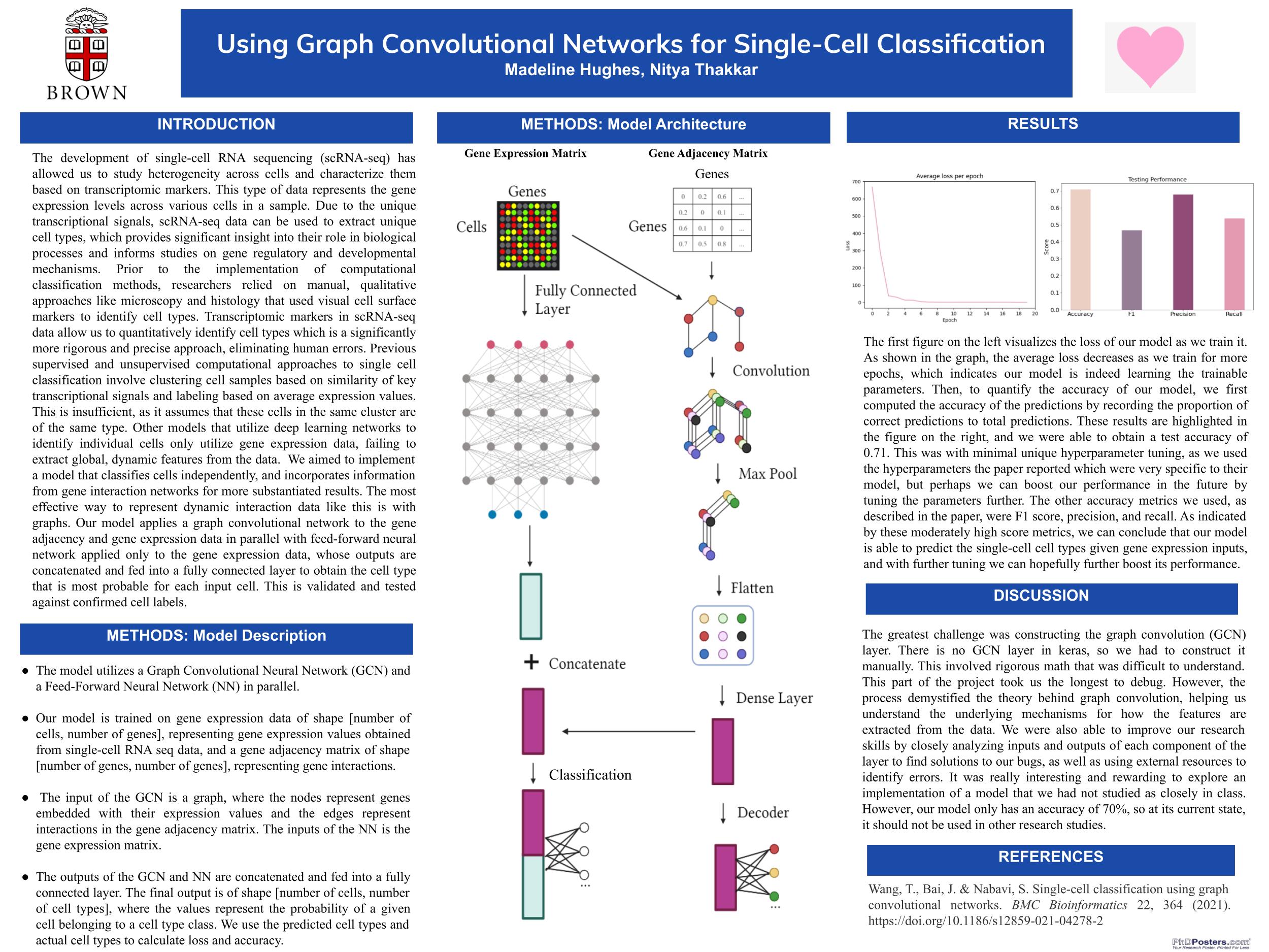
The first figure on the left visualizes the loss of our model as we train it. As shown in the graph, the average loss decreases as we train for more epochs, which indicates our model is indeed learning the trainable parameters. Then, to quantify the accuracy of our model, we first computed the accuracy of the predictions by recording the proportion of correct predictions to total predictions. These results are highlighted in the figure on the right, and we were able to obtain a test accuracy of 0.71. This was with minimal unique hyperparameter tuning, as we used the hyperparameters the paper reported which were very specific to their model, but perhaps we can boost our performance in the future by tuning the parameters further. The other accuracy metrics we used, as described in the paper, were precision, recall, and F1 score. Precision is the ratio of true positive scores to the total number of true and false positives. Recall is the ratio of true positive scores to the total number of true positives and false negatives. The F1 score is the weighted average of the precision and recall scores. As indicated by these moderately high score metrics, we can conclude that our model is able to predict the single-cell cell types given gene expression inputs, and with further tuning we can hopefully further boost its performance.

Discussion, Challenges, Future Work

The greatest challenge was constructing the graph convolution (GCN) layer. There is no GCN layer in keras, so we had to construct it manually. This involved rigorous math that was difficult to understand. This part of the project took us the longest to debug. However, the process demystified the theory behind graph convolution, helping us understand the underlying mechanisms for how the features are extracted from the data. We were also able to improve our research skills by closely analyzing inputs and outputs of each component of the layer to find solutions to our bugs, as well as using external resources to identify errors. It was really interesting and rewarding to explore an implementation of a model that we had not studied as closely in class. However, our model only has an accuracy of 70%, so at its current state, it should not be used in other research studies.

We hope to further tune our model so we can improve its performance to match the paper’s performance, keeping in mind that we are using both a different dataset and a different framework (Tensorflow rather than PyTorch). We hypothesize that the paper finely tuned their model to perform really well on their datasets, which is why our performance may not be as great on theirs using the same hyperparameters. We also hope to test this model against another version of the model that has no encoder/decoder layers and instead is just a simple feed forward network; we hypothesize that it will not perform as well without the encoder output, but hope to test it to validate the effectiveness of this model approach.

An interesting addition to this model would be if it could incorporate information about cells’ spatial locations in a tissue. This could allow for interesting developments downstream with understanding intercellular interactions.

Reflection

Our project ultimately turned out much better than expected, because we chose a complicated model to implement. We were hoping to get our model to run with an accuracy that was above 50% and we accomplished that, yielding an accuracy of 71% on our final run. At first, we tried to follow other graph convolution tutorials due to the complexity of the computations described in the paper, but ultimately followed the paper’s mathematical method because we ran into many errors and the model wouldn’t function properly. If we had done our project over again, we would have outlined our understanding of the architecture before starting, as we just started coding following their architecture depiction and likely wasted a lot of time on the bugs that were derived from misconceptions. Our accuracy could definitely be improved, as the latest run is approximately 71%. We could potentially improve this accuracy by adding more layers and tuning hyperparameters like the learning rate, batch size, feature space, and number of epochs. The biggest takeaway from this project is how it demystified the process of computational research. We gained more insight into how researchers find projects in the literature that they want to work on and where they begin. We were always intimidated by the gap between academic coding projects and professional research endeavors, but completing this project gave us more confidence in our abilities and fueled our interest in a research career.

Link to final write-up

Link to reflection

Link to initial outline

Built With

• keras
• python
• tensorflow