-

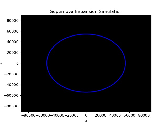
This particular Type II supernova blast is in its Sedov-Taylor expansion phase. Radial expansion has already significantly slowed.
-
Later in the supernova radius lifespan, expansion will have slowed even further. The radius has entered its "snowplow" phase.


Inspiration
Our team had never met prior to the Hackation however after our introductions, we realized we had a common interest in modelling astrophysical motion! Hackathons are a perfect opportunity to showcase skills, both technologically and academically. As people who have a genuine passion for physics and coding, this opportunity was an amazing find for us, and we were lucky to find incredible teammates who are just as enthusiastic as we were. In particular, we wanted to delve into a sophisticated topic, which is (in our case) modelling the time evolution of a Type II Supernova blast radius.
What it does
Our project simulates a Type II Supernova blast radius over time. The first half of our project is an Interactive Jupyter Notebook file that allows the user to simulate blast radii for various time periods, and stars of various masses as well. The user can interact with this application via two sliders (one for time in years, one for mass in number of solar masses). The user can then examine how the blast radius changes over time (i.e. how the speed decreases over time).
The second half of our project is a full animation depicting the evolution of a SNR over its 4 primary phases. For each phase, the plot changes color to allow for better identification.
How we built it
This project was divided into two portions, both coded with Python. We used the libraries "numpy" and "matplotlib". We started by building the animation, and we built our interactive application off of this template, using the "ipywidgets" package.
import numpy as np
import matplotlib.pyplot as plt
from ipywidgets import interactive
A good amount of time for this project was spent calculating the relevant constants and coefficients for our simulation. These included proportionality constants for calculating the blast radius at a given point in time.
lightSpeed = 3 * 10**8
ejectVel = lightSpeed / np.sqrt(50)
ismDensity = 1.66 * 10**-20
heatRatio = 1.625

sedovTaylor = ((0.75 / 16) * (lightSpeed**2 / (np.pi * heatRatio * ismDensity))) ** 0.2
snowPlow = 1.62 * 10 ** 7
pDrive = 87089.51
sunMass = 1.989 * 10**30
Assuming that the local interstellar medium has a uniform density distribution, a parametrization of the blast radius can be seen as a perfect circle (as viewed from a cross-section with a point on the z-axis). That is, let x(t) = R(t) * cos(t) and y(t) = R(t) * sin(t), for t ranging from 0 to 2 * pi. Because t is an independent variable (unlike x and y, which depend both explicitly and implicitly, through R(t), on t), we can define it right away.
t = np.linspace(0, 2 * np.pi, 100)
The radius of a supernova remnant depends on two parameters: time and mass. Depending on the phase of the remnant, its radius will be proportional to various powers of time i:
def radius(i, m):
    rFreeToSedov = (sunMass * m) ** 0.3 * ejectVel * 1000
    rSedovtoPlow = (sunMass * m) ** 0.2 * sedovTaylor * 9000 ** 0.4
    rPlowtoDrive = snowPlow * 240000 ** 0.3
    if i <= 1000:
        r = (sunMass * m) ** 0.3 * ejectVel * i
    elif 1000 < i <= 10000:
        rInit = rFreeToSedov
        r = rInit + (sunMass * m) ** 0.2 * sedovTaylor * (i - 1000) ** 0.4
    elif 10000 < i <= 250000:
        rInit = rFreeToSedov + rSedovtoPlow
        r = rInit + snowPlow * (i - 10000) ** 0.3
    else:
        rInit = rFreeToSedov + rSedovtoPlow + rPlowtoDrive
        r = rInit + pDrive * (i - 250000) ** 0.25
    return r
The supernova was plotted using the given radius:
def supernova(time, mass):
    x = radius(time, mass) * np.cos(t)
    y = radius(time, mass) * np.sin(t)
    plt.plot(x, y)
    print("Blast Radius: " + str(radius(time, mass) / 1000) + " km")
    plt.title('Supernova: A Super Nova Thing!')
    plt.savefig('supernova')
We added user-interactivity with the following code:
superPlot = interactive(supernova, time=(0, 750000, 1), mass=(1.4, 200, 0.1))
superPlot
The final result is saved as an Interactive Jupyter Notebook, which is available on GitHub.
Challenges we ran into
One of the hardest parts of coding this project was accounting for the incredibly large (and small) relevant values in this problem. For instance, it was initially difficult to effectively model all phases of the supernova blast radius because some phases were very short in duration, in relation to other phases. As such, we had to find a workaround, adjusting our time scale for our animation. In addition, we also thought about how to make our interactive application as easy to use as possible for the user.
In terms of the physics, calculating the time periods over which the phases of the SNR exist was the most challenging. For the first phase, the calculation was quite straight forward. However, for the second phase, we had to calculate the approximate temperature of the SNR as a function of the star’s initial mass and use the temperature when ions recombine into atoms to solve for time. At this point, the expansion ceases to be adiabatic and changes into the next phase.
Accomplishments that we're proud of
Over a very short time period, we were able to vastly deepen our understanding of SNRs and write a code which models their evolution! None of us would have been capable of doing so alone.
This was the first project that many of us have ever coded completely from scratch. Furthermore, we were able to implement a user-interactive learning tool about a sophisticated physics topic. We are particularly proud of our degree of accuracy when calculating and simulating the motion of the supernova blast radius. Moreover, this is a project that allowed us to demonstrate our Python coding skills, as well as our understanding of Python's capabilities and our ability to adopt the mindset of physicists and programmers simultaneously.
What we learned
Firstly, we obtained a high degree of exposure to not only Python coding, but also its common packages like "numpy" and "matplotlib". Their computational and simulation abilities are incredible, as we were able to explore through our project. Furthermore, not only did we develop a solid skill set in Python this weekend, but we also learned quite a bit about a new topic that none of us have ever learned in lectures before.
We learned about the multiple phases to a SNR’s expansion. We learned new techniques that allow one to solve for blast wave radii and about the density of the Interstellar medium. In addition, we were able to share knowledge with each other, such as how to animate a plot in Python in a physics context!
We strongly believe that this Hackathon was a success for our team, because we obtained new knowledge and skills that we can take with us wherever we go.
What's next for Type II SNR Modeller
In the future, we hope to come back to this project and add more elements. For instance, we could add heat maps, pressure distributions, energy distributions, and countless other visualizations of relevant data. More and more, even though a solid understanding of analytical methods is crucial, complicated physics problems rely on numerical methods to be solved. As such, the significance of computer science in physics can only grow from here. We hope to be able to continuously improve upon our Type II SNR Modeller, contributing to the joint computer science and physics community.


Log in or sign up for Devpost to join the conversation.