Inspiration

As a research associate in a biotech startup, I have screened nanobodies in the lab. A single round takes up to a week, and hours of hands-on work go into each one. Affinity maturation (turning a weak binder into a strong one) means repeating that cycle again and again, and almost everything you grow and sort gets washed away. Shortening the process is worth real time and real reagent.

We found a preprint from the Debora Marks Lab, Paul et al. (2026), Machine learning enables efficient and effective affinity maturation of nanobodies (bioRxiv). It shows that a model trained on sequencing counts from an early selection round can predict which variants enrich in later rounds. The method works and the authors released their data under an MIT licence — but it ships as research code built around their own three campaigns, with the analysis spread across notebooks and scripts. Nobody who is not already a computational biologist is going to run it.

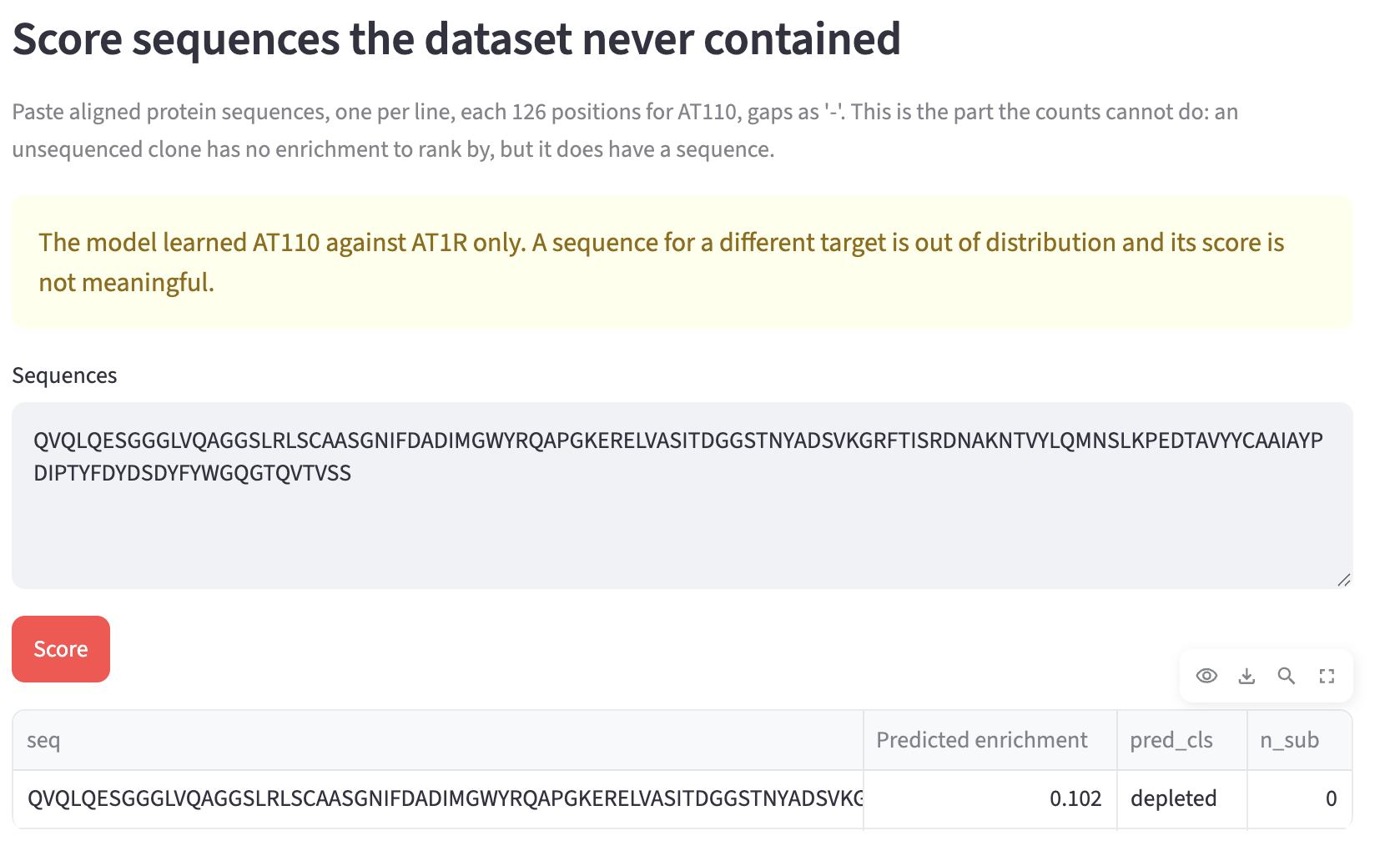
So we built the tool that method deserves: an application where you load one round of sequencing, see your enrichment computed in front of you, see how well a model trained on it actually performs, read off which substitutions it has learned to favour, and paste in your own designed sequences to have them scored. It can run on your own data, in about five seconds, on a laptop.

What it does

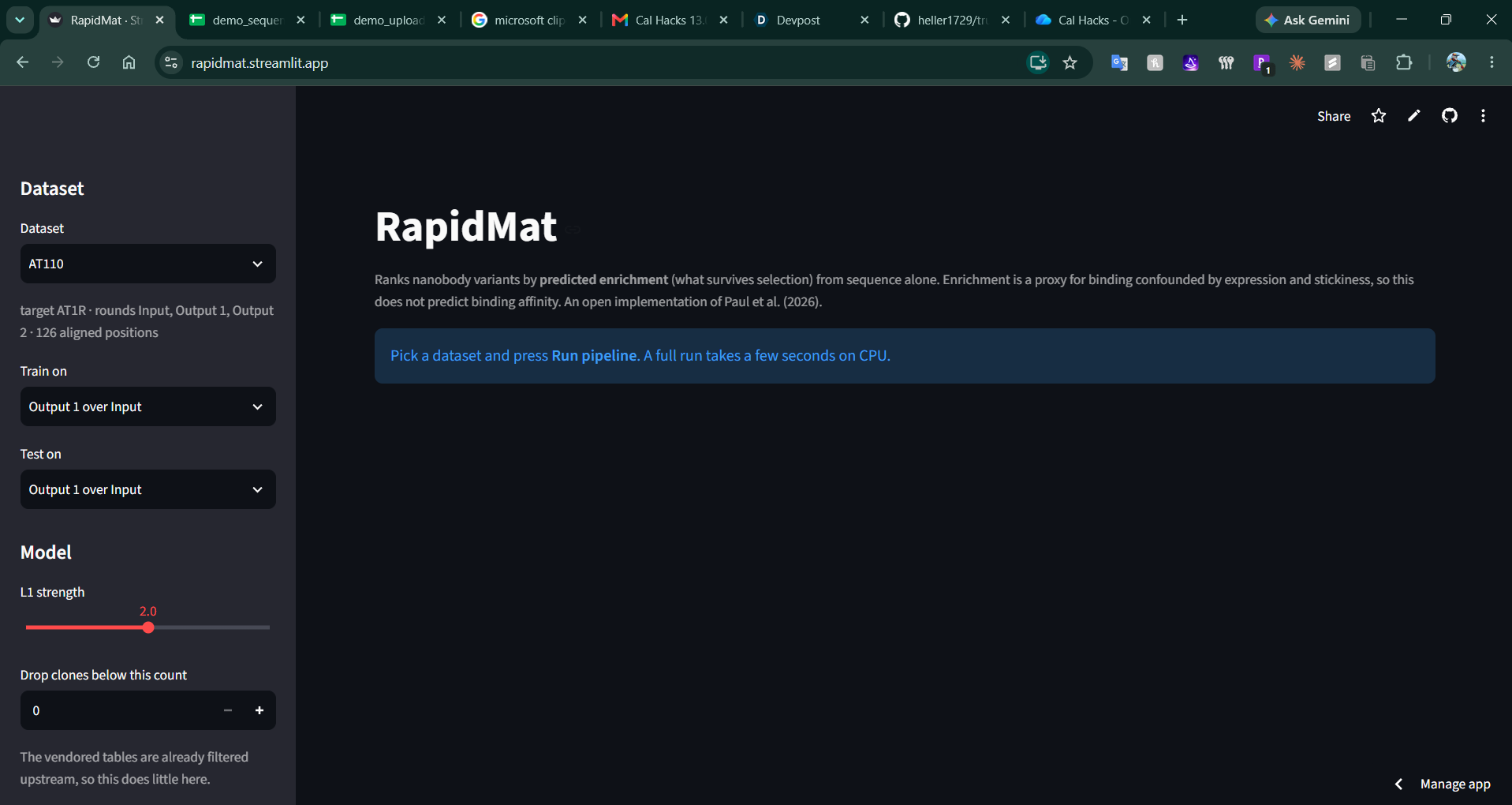
Takes one screen. An input library and the output of a single selection round. That is what a real campaign has in hand after one week, and it is deliberately all RapidMat asks for.

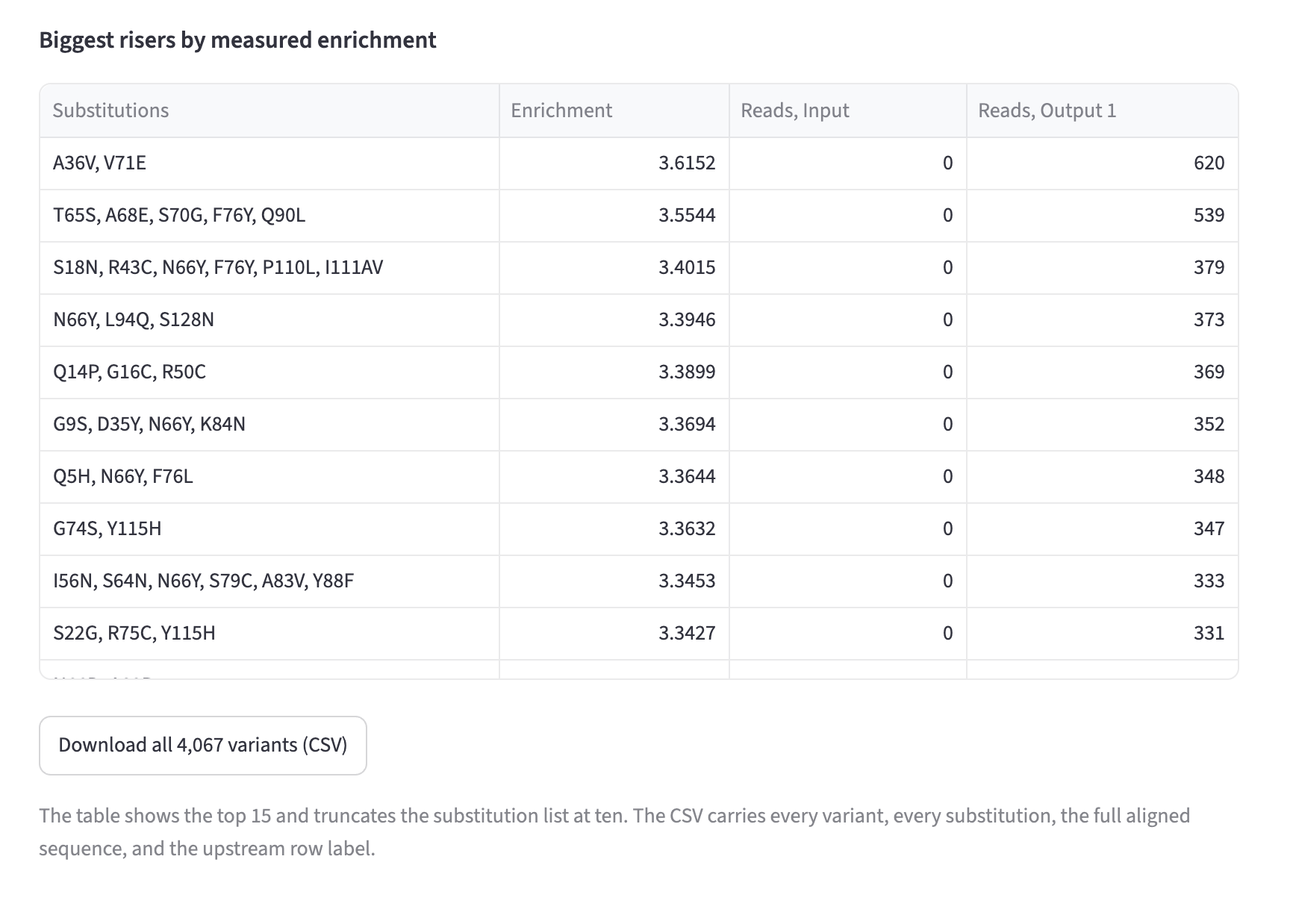
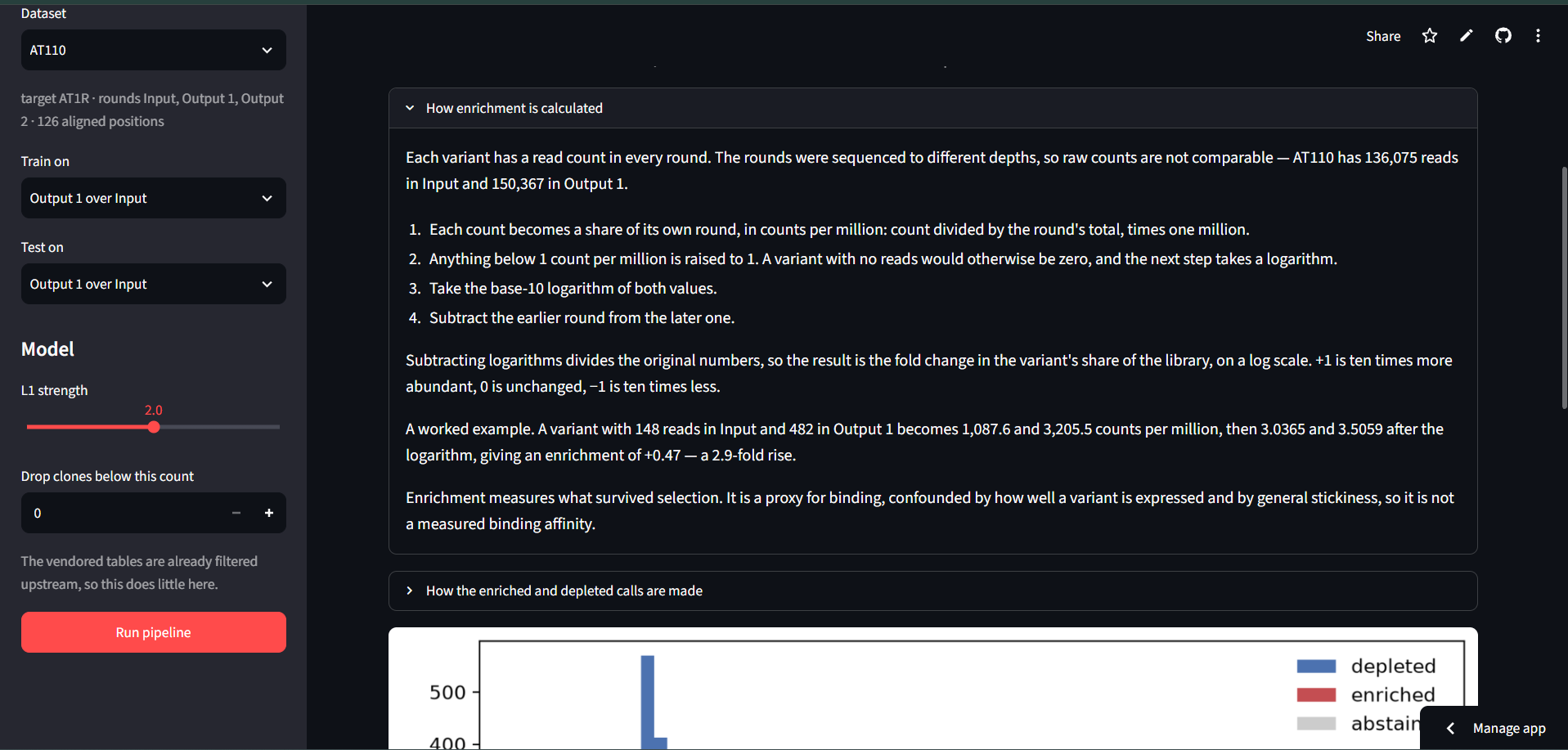
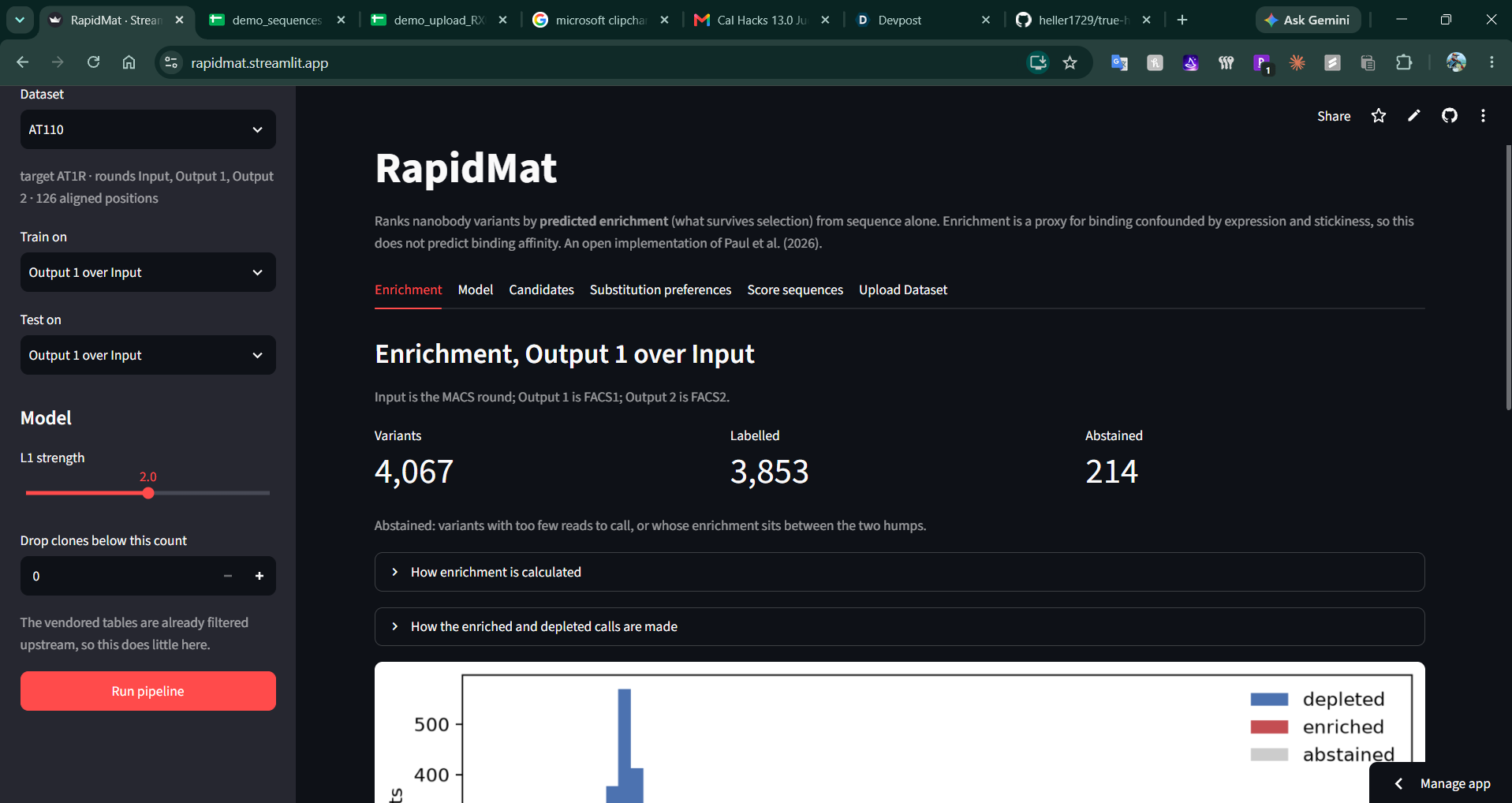
Computes enrichment and shows the arithmetic. Counts become counts per million, get a detection floor, go through a log, and the earlier round is subtracted from the later one. The app explains each step in plain language with a worked example from the loaded dataset, because a scientist should not have to trust a number whose derivation is hidden.

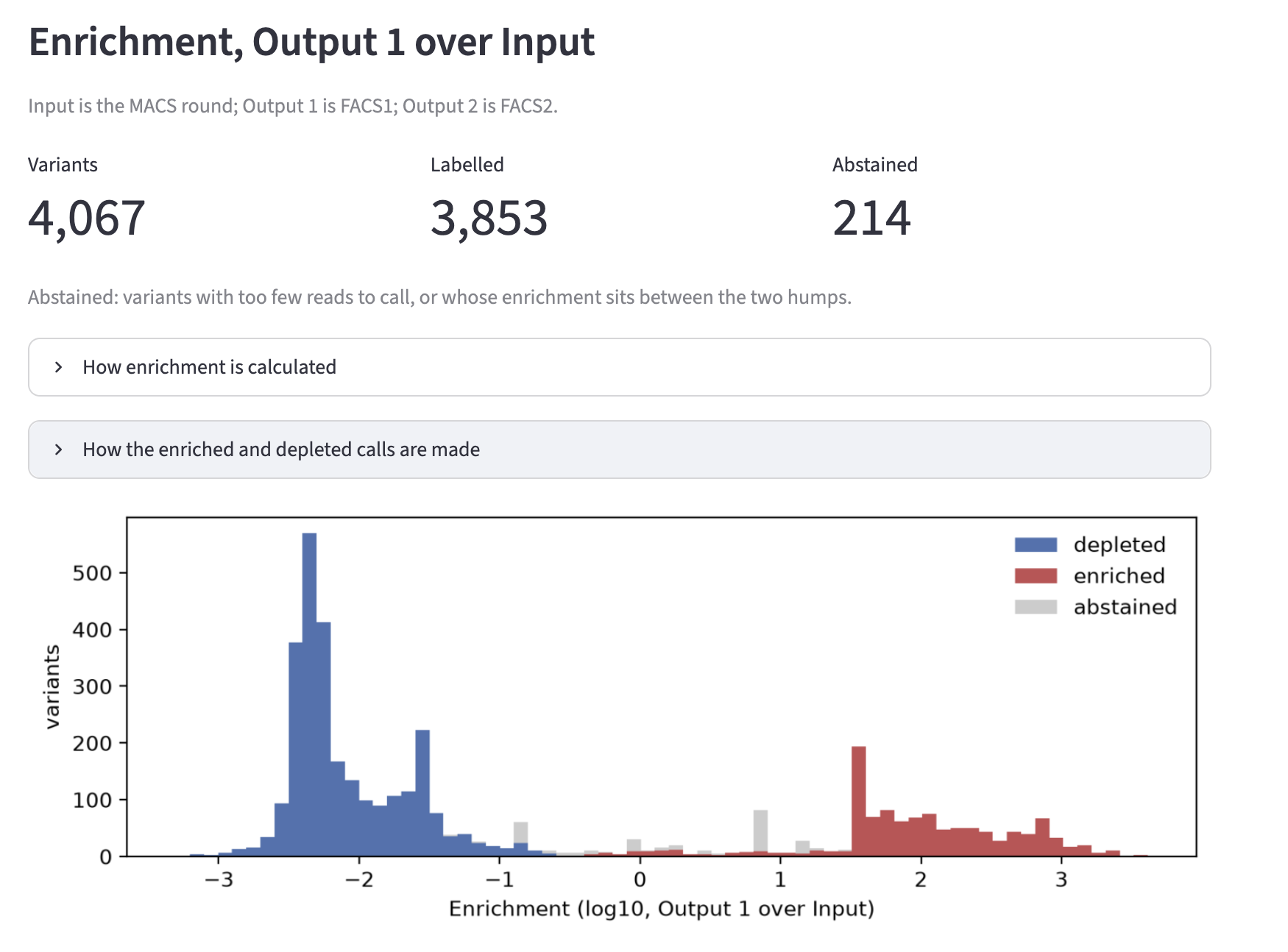
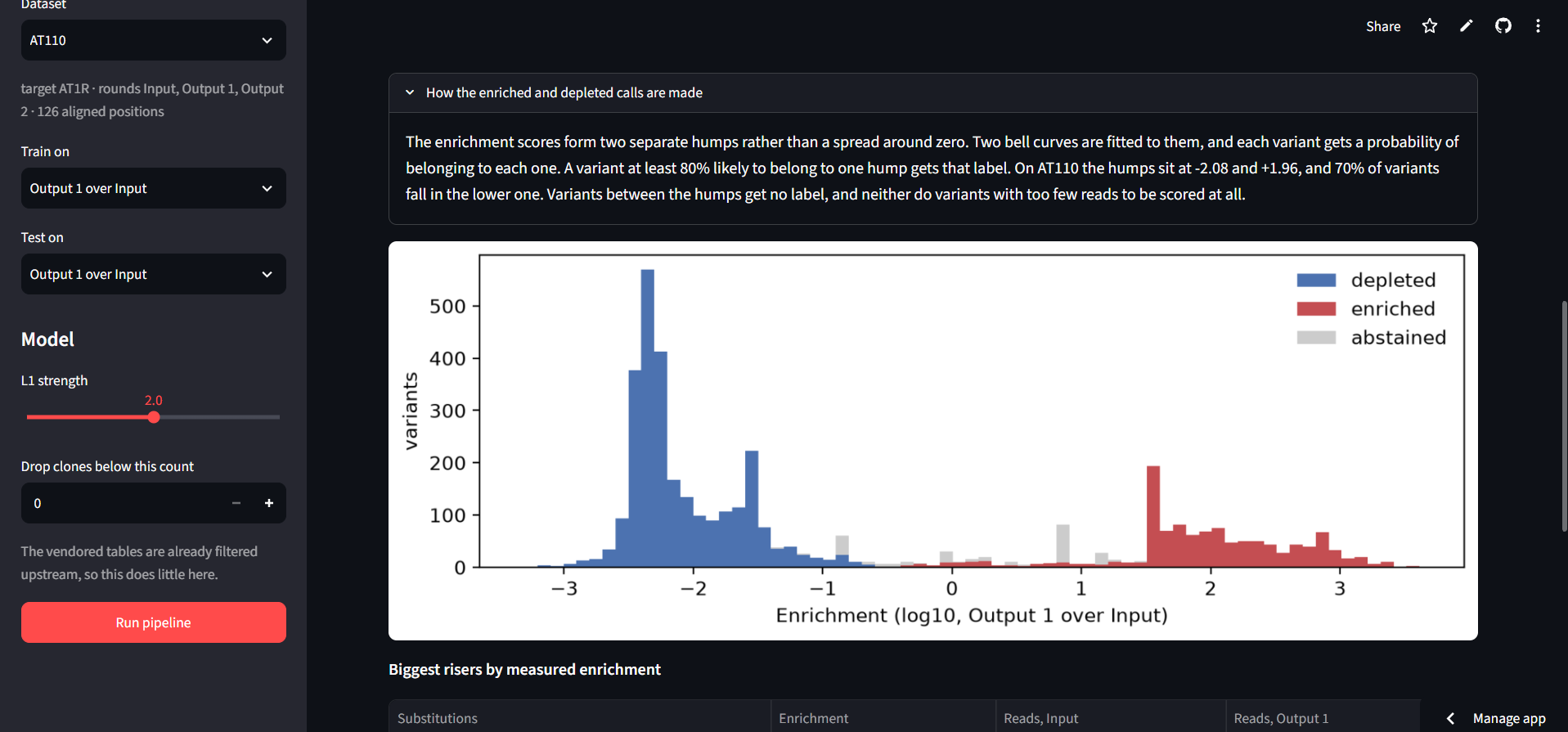
Calls winners and losers Enrichment scores fall into two humps rather than spreading around zero, so a two-component mixture is fitted and lets the data place the boundary. Variants that sit between the humps are left uncalled rather than forced into a class, and the app says how many and why.

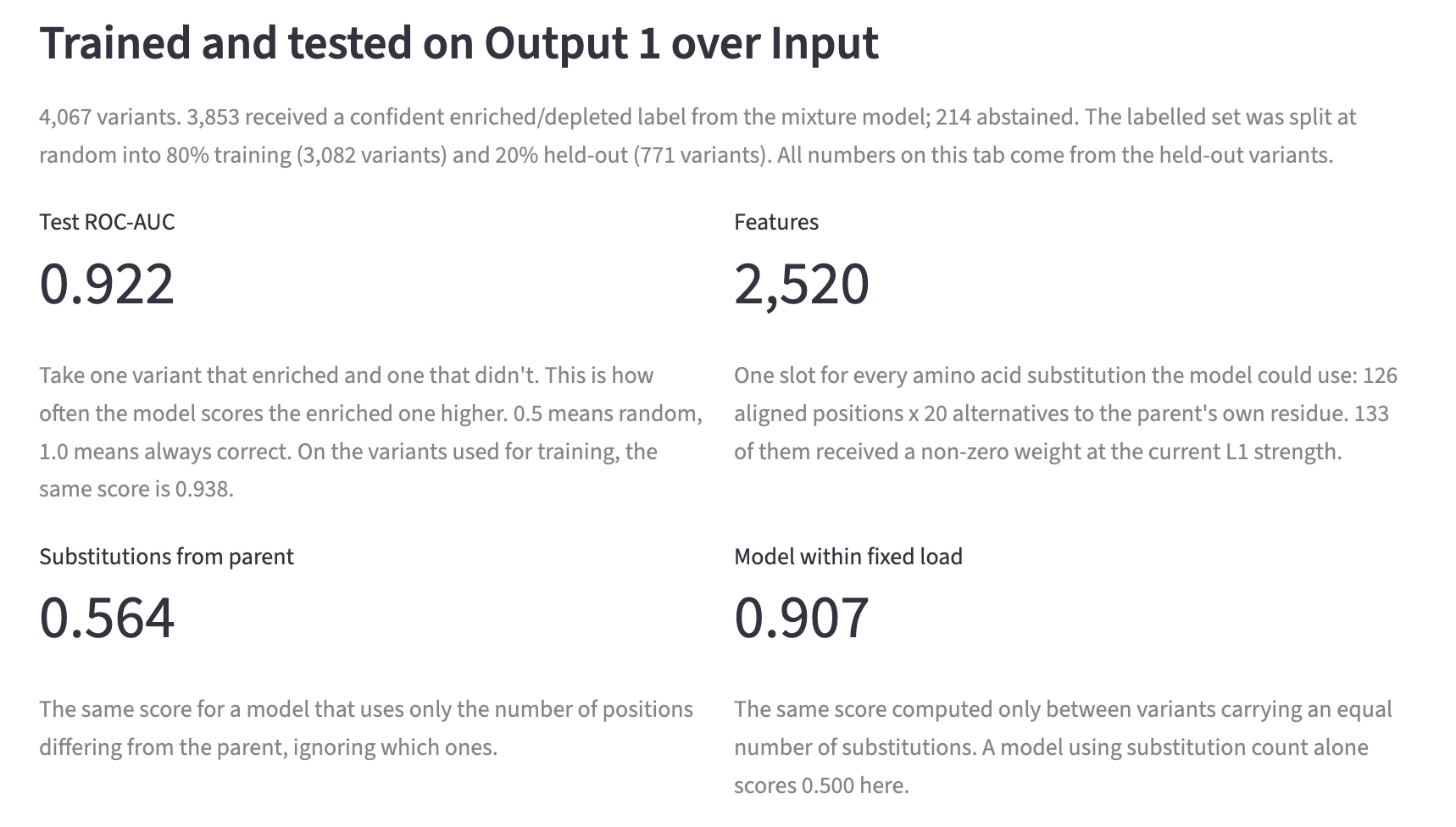
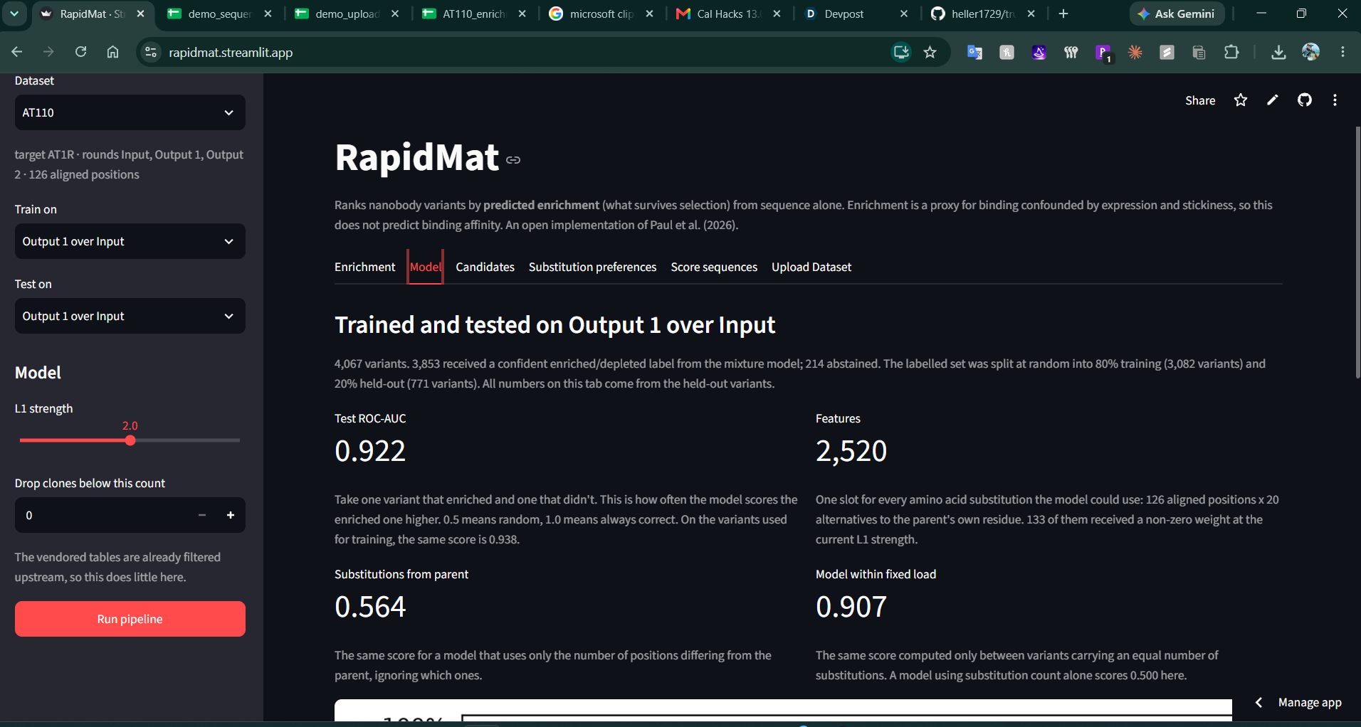
Trains and honestly tests a model. Features are per-substitution indicators; the label is the enrichment call. It reports accuracy on held-out variants, alongside the sequence-only baseline it has to beat (ranking by how many mutations a variant carries). On AT110 the model reaches 0.922 ROC-AUC against 0.564 for that baseline.

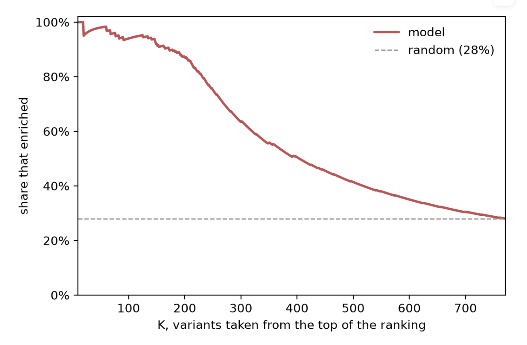
Says how many of your top picks are real. A precision-at-K curve answers the question a bench scientist actually has: of the top 50 candidates in the test set, 98% genuinely enriched, against 28% from picking 50 at random.

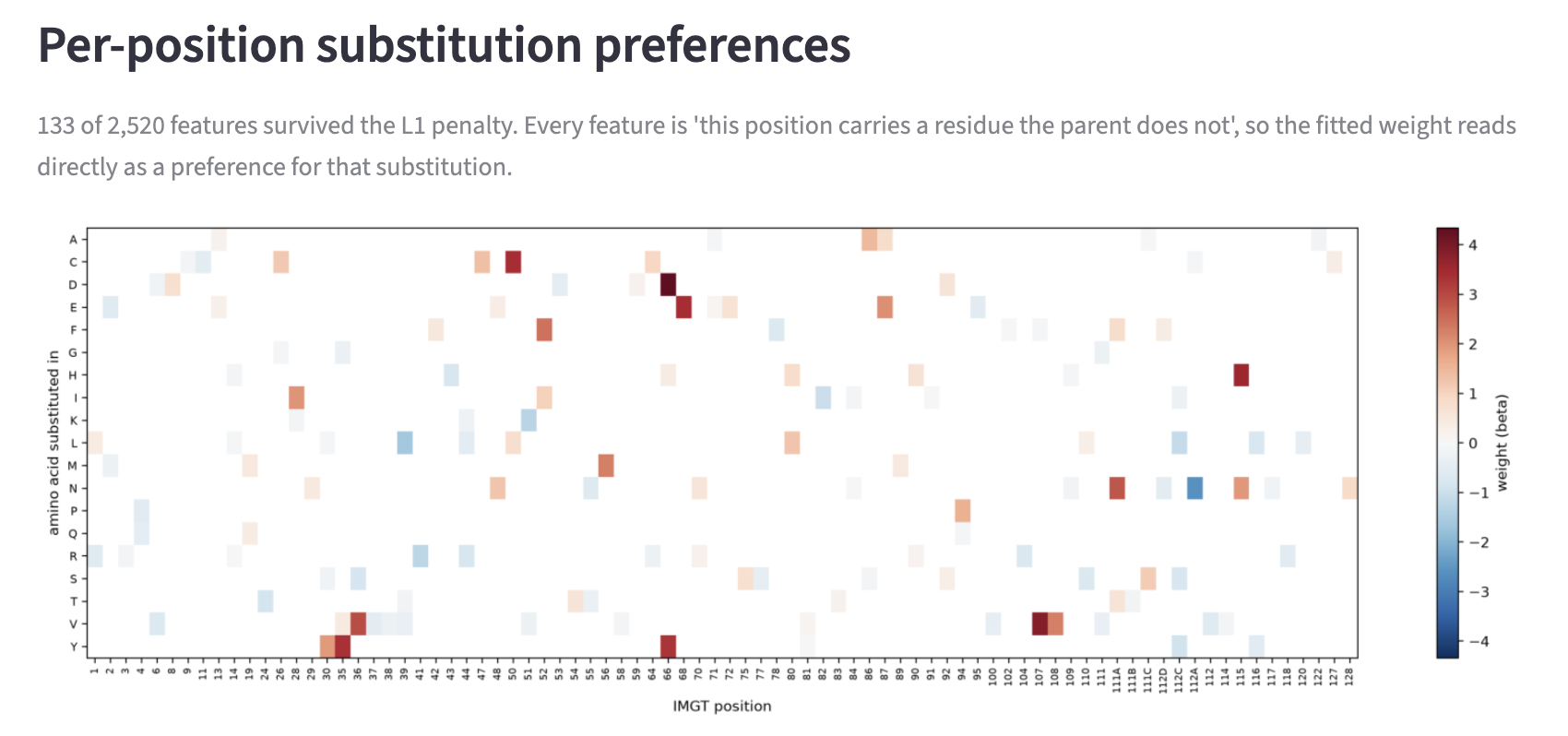
The substitution design map. Every fitted weight is one amino acid substitution at one position. There are no hidden layers to hide behind. You can read the strongest substitutions straight off the map and build the next variant from them.

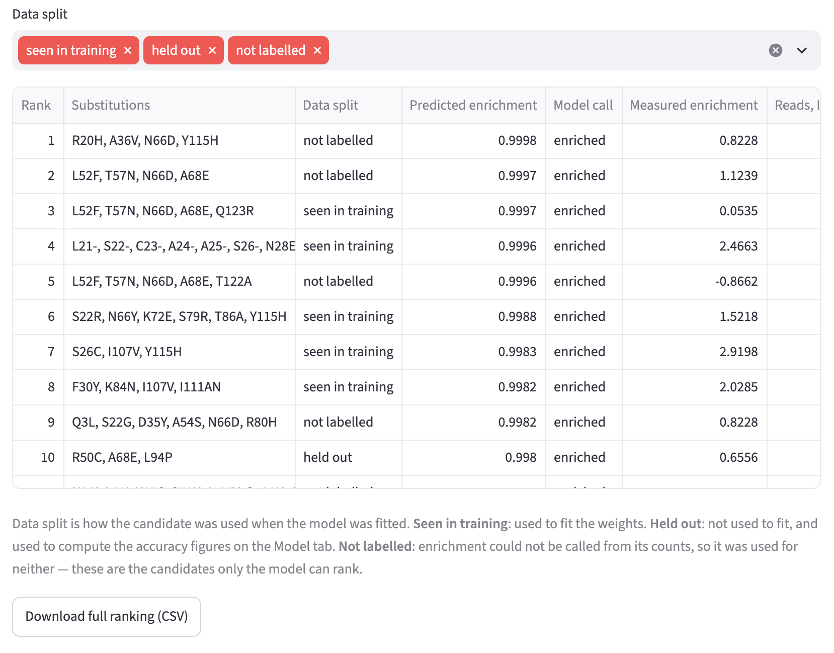
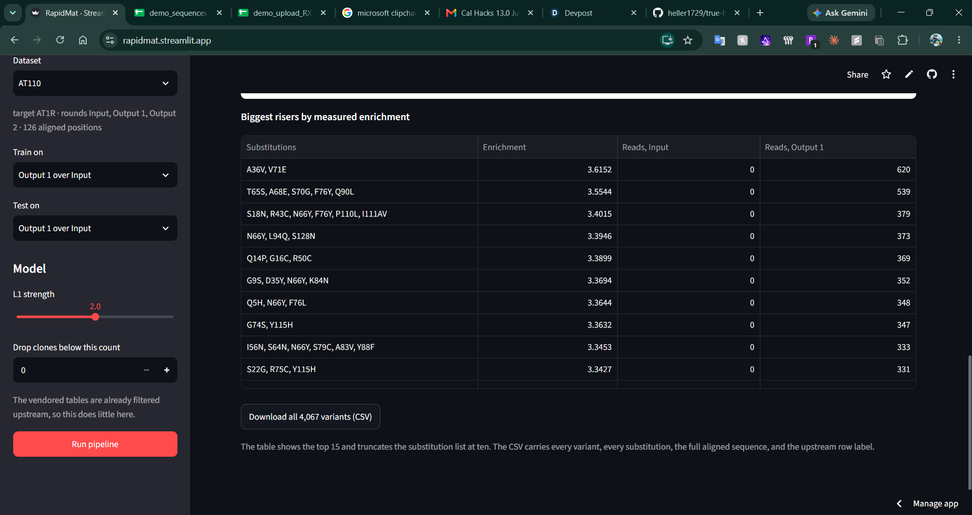
Marks which scores it had already seen. Every candidate is labelled as used in training, held out, or never labelled at all, and the table can be filtered to just the ones the model did not train on — 985 of them on AT110.

Rescues clones the counts cannot rank. 214 variants on AT110 have no enrichment call at all, either because their log ratio came out exactly zero or because the mixture was less than 80% sure. They still get a sequence-based score, so scientists can easily order the top sequences even without enrichment data.

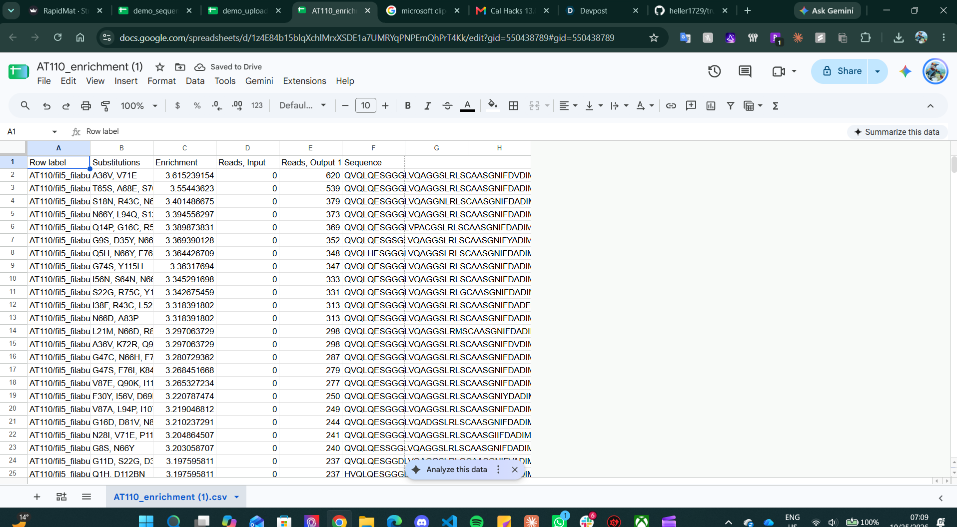
Runs on your own data. Upload a CSV of clone IDs, aligned sequences and per-round counts and every tab populates from it — the same enrichment, the same model, the same map. No reformatting into anyone's internal schema. We tested it by handing the app a demo dataset different from the default used to validate it (RX002).

How we built it

Recovering the recipe. The preprint describes its method; the exact arithmetic lives in the authors' code. We read it out and reproduced it. The pre-filter library sizes are from the normalised columns.

Model Features and Representation The aligned sequence is one-hot encoded with the parent's own residue dropped at every position. Every weight reads as a preference for a specific substitution, and the design map represents this. L1-penalised logistic regression on AT110 keeps 133 of 2,520 candidate substitutions and zeroes the rest, so what comes out is a short list a scientist can act on instead of a dense matrix of noise.

Generality by construction, not by special case. Rounds are named by position — the first is Input, the rest are Output 1 onward — so the same code describes a three-round campaign, a five-round campaign, and a two-column uploaded CSV. An uploaded dataset returns the same result object the built-in default campaign does.

Architecture app.py is purely a renderer. There is no Streamlit import anywhere inside the analysis package; everything goes through one call that returns a plain result object, so a web API and a different frontend can sit on the same pipeline later.

Tested. 142 tests. They load all three campaigns from the vendored data and assert the reproduction numbers, so the suite fails loudly if the recipe drifts. Against the authors' own fitted parameters we get coefficient sign agreement of 1.000 and Pearson r of 0.983; on their train/test configuration we reach 0.960 ROC-AUC against their published 0.964.

Challenges we ran into

Choosing a validation that matches reality. The paper trains on one round pair and tests on a later one, which is the stronger scientific check — but a user with one screen has no later round to test against. We made the app default to the configuration a real user actually has, and validated using a train/test split so the user can understand the accuracy of the model in their particular dataset.

Data leaking between rounds. The released tables carry one row per variant across all rounds, so asking for an early round pair still returned 1,190 variants that existed only because a later round had been sequenced. They were sitting at the top of the ranked candidate list. Filtering to the rounds actually selected fixed it and moved no accuracy number, because those rows had never been in training or testing in the first place.

Generalising a pipeline built for one dataset. Round names, alignment widths and file layouts were assumed throughout the original code. Removing those assumptions was most of the work in making the tool accept anyone's data.

Making it usable for a scientist. Internal field names, assay-specific round labels, and a row identifier in the column where a sequence belonged. A model that a biologist cannot interrogate is a model a biologist should not trust, so we made sure to be clear and transparent about what each number means and how it was calculated.

What we learned

Jessica: I came in as the biologist and learned a great deal about how modelling actually works; it was an amazing experience implementing models I learned in class on real data, in a way that's provably useful. Getting to troubleshoot when the model didn't work as expected and exploring what each metric meant was, well, deeply enriching. Also learned more about structuring pipelines.

Pratham: On the bio side I basically learned the whole selection process from scratch, how you take a weak binder and improve it over rounds, and what measuring enrichment means.

What is next for RapidMat

Sequence alignment inside the tool, so data does not have to arrive in such a narrow format. This reduce the barrier to someone using RapidMat on their own data, and it would let the whole sequencing analysis run end to end in one place.
A signal for substitutions the library never sampled, drawn from chemical similarity to what it did see, so a designed variant at an unexplored position gets an informed estimate rather than silence.
Separating binding from growth. Some clones rise across rounds because they replicate faster, not because they bind better. Flagging those is the scientifically most interesting extension.