Toronto Shelter Signal - Team 6

About the project

Try it out: https://public.tableau.com/app/profile/marcello.marcello5067/viz/SDSS_T6/Dashboard12?publish=yes

Inspiration

Toronto’s shelter system often operates close to capacity. We wanted to turn open data into something operationally useful: where is the system most strained, when does it worsen, and can we recommend lower-occupancy options to support “spreadness” (load balancing)?

What we built

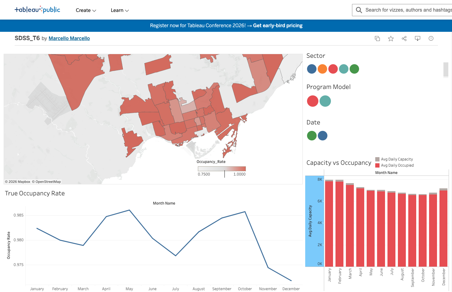
We built ShelterPulse Toronto: an end-to-end pipeline that cleans and aggregates shelter occupancy data, visualizes trends and hotspots, trains a model to predict occupancy, and evaluates whether the model can support daily routing decisions.

We focused on two outputs: 1) Awareness: “who/where/when/what” drives high occupancy (sector, geography, seasonality, program area). 2) Spreadness: a predictive ranking tool that recommends the Top-K least-full options for a given day.

How we built it

1) Data cleaning

Standardized postal codes (uppercase, remove whitespace) and removed invalid/missing entries.
Aggregated duplicate rows into a stable unit defined by
[ (\text{date}, \text{postal}, \text{sector}, \text{service type}, \text{program model}, \text{program area}, \text{capacity type}) ]
Recomputed: [ \text{Occupancy Rate} = \frac{\text{Occupied Capacity}}{\text{Actual Capacity}} ]

2) Awareness analysis

Converted postal codes to FSA (first 3 characters) for consistent area-level aggregation and mapping.
Built charts for 2025 occupancy by sector, program area, and month (seasonality).
Optional geo-visualization: merged FSA boundaries with aggregated data to create an interactive choropleth.

3) Modeling for “Spreadness”

Features: encoded categorical program identifiers + calendar features (month, day of week).
Model: HistGradientBoostingRegressor to predict OCCUPANCY_RATE, with guardrails by clipping predictions to ([0,1]).

4) Evaluation We evaluated the model in four ways:

Core metrics: MAE, RMSE, and sanity checks with predicted-vs-actual and residual plots.
Error slicing: MAE by sector, capacity type, and near-full status ((\ge 0.95)).
Ranking metrics for load balancing: Top-K capture + regret compared to an oracle ranking. [ \text{Regret} = \overline{y_{\text{true}}(\text{Predicted Top-K})} - \overline{y_{\text{true}}(\text{Oracle Top-K})} ]
Feature importance: permutation importance to verify the model is learning sensible drivers (location and program type dominate, weekday is minimal).

What we learned

In a near-capacity system, ranking quality matters more than perfect point prediction. Measuring Top-K performance + regret is a better evaluation for load balancing.
Error slicing revealed that performance differs across sectors and that “near-full” cases dominate the dataset—important for both interpretation and future model improvements.
Postal geography (FSA vs full postal code) is a practical tradeoff between map consistency and granularity.

Challenges

Imbalanced occupancy: most records are near full, so models can look good overall while struggling on rare low-occupancy cases (which are exactly the cases load balancing cares about).
Data granularity: no unique shelter ID, so aggregation decisions matter and can change the story.
Drift and operational changes: performance varies across time windows; we used walk-forward validation to test generalization.
Geospatial mapping: joining FSA codes to boundary files required extra preprocessing and careful handling of missing FSAs.