Inspiration
Cities are already losing \( 20\%–30\% \) of treated drinking water to “non-revenue water” from leaks and bursts, but most utilities only find the big failures after a street floods or a customer complains. We wanted to treat this like a signal-processing and physics problem instead of a manual search problem: there are already pressure waves flying through the system every time a pump shuts off or a valve moves. The question we asked was: can we turn those everyday events into a built-in sonar that points to hidden leaks without ripping up the street or blanketing the city in new hardware?
What it does
Concept Epsilon is a “Transient Forensics Engine” for water networks.
Given a digital model of a utility’s network and a few pressure sensors, it:
- Uses scheduled pump/valve events as excitation “pings” of the system.
- Reads the resulting pressure waves at the sensors (with wave speed \( a \approx 1000~\text{m/s} \)).
- Runs a physics-guided ML model to infer which pipe segment is leaking (or that there is no leak).
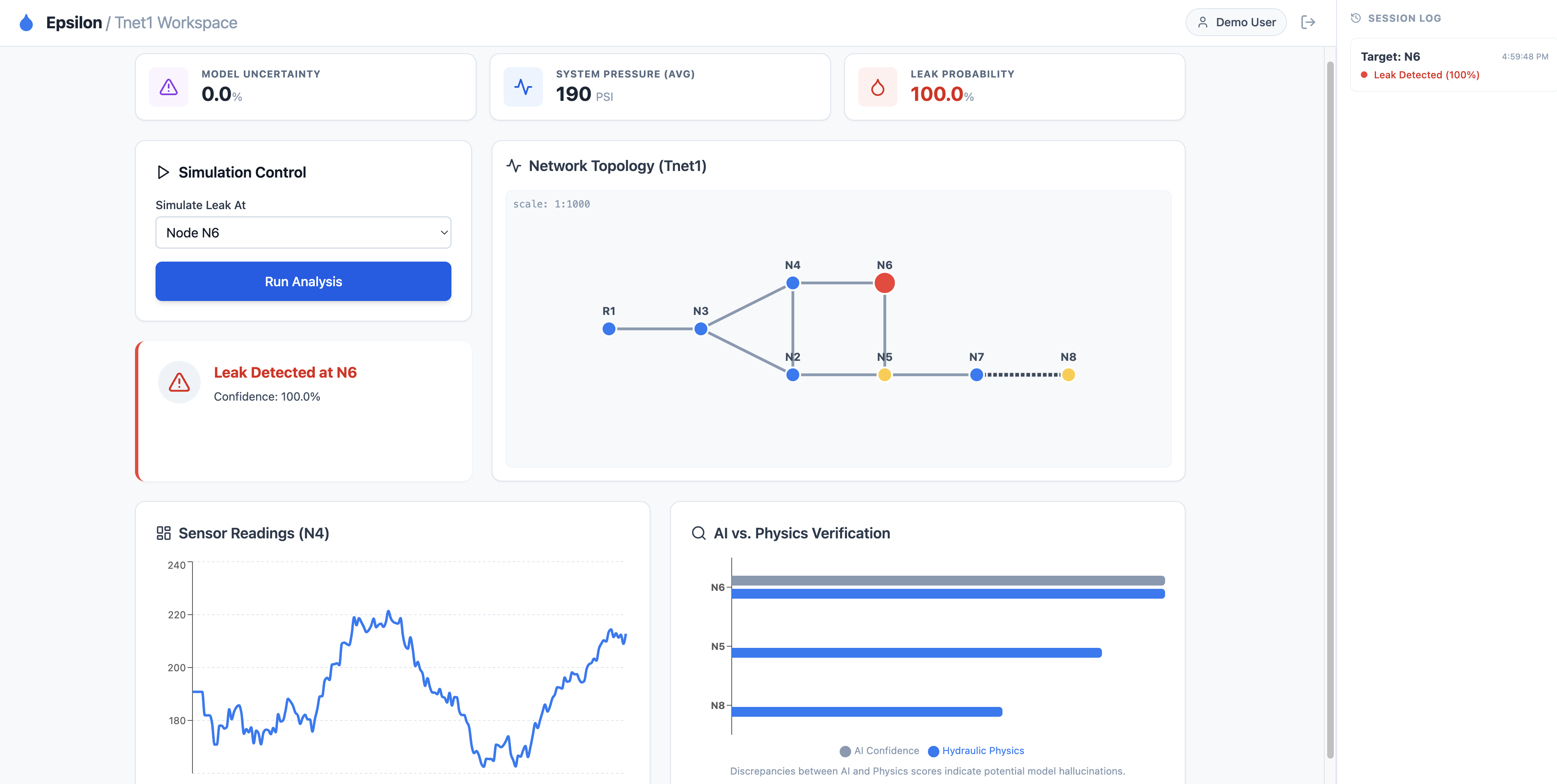
- Cross-checks the AI prediction against a full transient simulation and only reports leaks that are physically consistent.
The output for operators is a ranked list of suspect pipes and a map-based view of the incident they can act on immediately.
How we built it
- Digital twin and physics core – We start from an EPANET network model and wrap it with TSNet to simulate full transient hydraulics. Each pipe is modeled with the 1D water-hammer equations for hydraulic head \( H(x,t) \) and discharge \( Q(x,t) \):
$$ \frac{\partial H}{\partial t} + \frac{a^{2}}{gA}\frac{\partial Q}{\partial x} = 0, \qquad \frac{\partial Q}{\partial t} + gA\frac{\partial H}{\partial x} + \frac{f\, Q\lvert Q\rvert}{2 D A} = 0 $$
where \( a \) is the wave speed, \( A \) the pipe area, \( D \) the diameter, \( g \) gravity, and \( f \) a friction factor. TSNet solves these hyperbolic PDEs with the Method of Characteristics to propagate pressure waves through the network.
- Synthetic leak library – A leak on a pipe is modeled as an orifice-type emitter boundary condition:
$$ Q_{\text{leak}} = C_e H^m, \quad m \approx 0.5 $$
so higher local head produces stronger outflow and stronger damping of the passing wave. For each candidate pipe and leak size \( C_e \), we inject this leak in TSNet, trigger a standard pump/valve event, and record high-frequency pressure traces at virtual sensors. Each run becomes a labeled example: multichannel pressure time series \( x(t) \in \mathbb{R}^{S \times T} \rightarrow \) true leak pipe index or “no leak.”
- Inverse model – We train a 1D convolutional neural network \( f_\theta \) that approximates the inverse map
$$ f_\theta : x(t) \longrightarrow p(y \mid x) $$
where \( p(y \mid x) \) is a probability distribution over all pipe segments plus a “no-leak” class. The CNN learns to use arrival times of reflections (\( t \approx L/a \)), phase shifts, and amplitude decay patterns to localize the leak.
Physics-consistency loop – At inference, the CNN proposes a small set of top-\(k\) leak candidates (pipes with highest predicted probability). For each candidate pipe \(p\), we:
- Run TSNet with a leak on pipe \(p\) (with a reasonable leak size) and simulate the same excitation event.
- Extract the simulated pressure trace \(x^{\text{sim}}_p(t)\) at the sensor and compare it to the observed trace \(x^{\text{obs}}(t)\).
We then compute a discrepancy metric, for example the mean squared error
$$ E(p) = \frac{1}{T} \sum_{t=1}^{T} \bigl(x^{\text{obs}}(t) - x^{\text{sim}}_p(t)\bigr)^2, $$
or equivalently use a correlation coefficient between \(x^{\text{obs}}(t)\) and \(x^{\text{sim}}_p(t)\).
If the best candidate’s error \(E(p)\) is below a threshold (and/or correlation is high enough), we accept that leak location; otherwise we treat the event as “no trustworthy leak prediction.” This way, the forward physics solver confirms or corrects the ML guess instead of blindly trusting it.
- Frontend + API – A backend service exposes endpoints to run scenarios and retrieve predictions, and a React frontend renders the network, incident scenarios, ranked leak candidates, and pressure traces for demo and operator workflows.
Challenges we ran into
- Data reality vs. simulation – Real utilities don’t have thousands of labeled transient events. We had to design a synthetic data pipeline rich enough to train ML but still grounded in realistic ranges for \( a \), \( f \), demand patterns, and leak sizes \( C_e \).
- Numerical stability – Transient simulations are sensitive to timestep \( \Delta t \), spatial discretization \( \Delta x \), and boundary conditions. Keeping the CFL condition \( a\,\Delta t / \Delta x \le 1 \) satisfied while injecting leaks and repeatedly firing events took careful configuration and debugging.
- Signal ambiguity – Different leak locations can produce deceptively similar pressure signatures \( x(t) \). Designing the CNN input windowing, normalization, and multi-sensor architecture to actually resolve those differences required several iterations.
- Bridging physics and UX – Turning raw PDE solutions and tensor outputs into a clean, intuitive UI for operators (who care about “which pipe do I dig?”) was non-trivial.
Accomplishments that we're proud of
- Built an end-to-end pipeline that goes from an EPANET file to a calibrated transient simulator, to a trained inverse model \( f_\theta \), to a working web demo.
- Demonstrated that using just a few sensors and a single excitation event, the system can narrow leaks down to a small set of candidate pipes on a realistic demo network.
- Implemented a physics-consistency check that significantly reduces “AI hallucinations” and forces predictions to pass a partial differential equation–based sanity check.
- Designed a map-based interface and scenario panel that lets non-ML experts explore incidents, view pressure traces, and see why the model is flagging certain pipes.
What we learned
- Physics-guided ML is more robust than either pure simulation or pure deep learning alone: the simulator encodes conservation laws and wave propagation, while the CNN handles the messy, nonlinear inverse mapping from \( x(t) \) to leak location.
- Framing matters: by treating routine operations (pump shutdowns, valve moves) as deliberate pings, we can extract much more value from existing infrastructure without demanding new hardware.
- Utility operators care less about model details and more about trust and workflow fit, which is why the explanation layer (waveform overlays, physics checks, and ranked candidates) is as important as raw accuracy.
- Building a realistic digital twin early forces better engineering decisions everywhere else in the stack.
What's next for Concept Epsilon
- Pilot with a real utility: Ingest a partner’s EPANET model and historical event/leak logs to calibrate the twin and test localization on past incidents, treating each incident as a labeled inverse problem instance.
- SCADA integration: Wire the engine into live pressure data streams so it can automatically flag anomalous events and propose leak candidates in near-real time.
- Generalization to other networks: Extend the same inverse-transient framework to district heating, gas distribution, and industrial pipelines—anywhere the 1D wave equations apply and leaks behave like dissipative impedance changes.
- Operational tooling: Add alert thresholds, reporting, and simple “playbooks” for field crews so the system fits directly into day-to-day operations, not just offline analysis.
Built With
- docker
- epanet
- fastapi
- git
- javascript
- leaflet-(or-similar-web-mapping)
- leaflet.js
- node.js
- numpy
- pandas
- python
- pytorch
- react
- tsnet
- typescript
- uvicorn
- vite
- vs

Log in or sign up for Devpost to join the conversation.