-
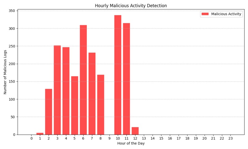
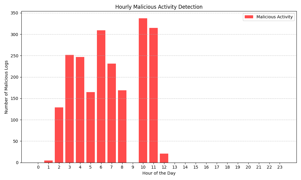
Graph of data
Step 1: Project Setup
Environment Setup:
- Install Python and necessary libraries. You can use Anaconda or a virtual environment.
- Install PyTorch:
bash pip install torch torchvision - Install additional libraries:
bash
pip install numpy pandas matplotlib scikit-learn
Prepare Your Workspace:
- Create a new directory for your project. Inside this directory, create subdirectories for:
- Data
- Notebooks (for Jupyter notebooks, if you prefer)
- Scripts (for your Python scripts)
- Create a new directory for your project. Inside this directory, create subdirectories for:
Step 2: Data Collection
Gather Network Traffic Data:
- You need historical network traffic data. If you don’t have access to real data, you can simulate it using random data or find datasets online (e.g., Kaggle, UCI Machine Learning Repository).
- Ensure your dataset contains time-stamped traffic volume data (e.g., packets per minute, bytes transferred).
Data Format:
- Your data should ideally be in CSV format, with columns for timestamps and traffic volumes:
timestamp, traffic_volume
2024-01-01 00:00:00, 150
2024-01-01 00:01:00, 200
...
- Your data should ideally be in CSV format, with columns for timestamps and traffic volumes:
Step 3: Data Preprocessing
- Load the Data: ```python import pandas as pd
# Load your dataset data = pd.read_csv('data/traffic_data.csv', parse_dates=['timestamp']) data.set_index('timestamp', inplace=True)
2. Visualize the Data:
   - Plot the traffic data to understand its trends.
   ```python
   import matplotlib.pyplot as plt

   plt.figure(figsize=(12, 6))
   plt.plot(data.index, data['traffic_volume'], label='Traffic Volume')
   plt.title('Network Traffic Over Time')
   plt.xlabel('Timestamp')
   plt.ylabel('Traffic Volume')
   plt.legend()
   plt.show()
- Normalize the Data:
- Normalize the traffic volume to help the model converge faster. ```python from sklearn.preprocessing import MinMaxScaler
scaler = MinMaxScaler() data['traffic_volume'] = scaler.fit_transform(data[['traffic_volume']])
4. Create Sequences:
   - Create sequences for RNN input. For instance, if you want to predict the next hour based on the last 10 minutes:
   ```python
   import numpy as np

   def create_sequences(data, seq_length):
       sequences = []
       labels = []
       for i in range(len(data) - seq_length):
           seq = data[i:i + seq_length]
           label = data[i + seq_length]
           sequences.append(seq)
           labels.append(label)
       return np.array(sequences), np.array(labels)

   seq_length = 10  # For 10 time steps
   X, y = create_sequences(data['traffic_volume'].values, seq_length)
Step 4: Splitting the Data
Split Data into Training and Test Sets:
train_size = int(len(X) * 0.8)  # 80% training data
X_train, X_test = X[:train_size], X[train_size:]
y_train, y_test = y[:train_size], y[train_size:]
Reshape for RNN:
- RNNs expect input in the form of (batch_size, sequence_length, features).
python
X_train = X_train.reshape((X_train.shape[0], X_train.shape[1], 1))  # Add feature dimension
X_test = X_test.reshape((X_test.shape[0], X_test.shape[1], 1))
- RNNs expect input in the form of (batch_size, sequence_length, features).
Step 5: Build the RNN Model
- Define the RNN Model: ```python import torch import torch.nn as nn
class SimpleRNN(nn.Module): def init(self, input_size, hidden_size, output_size): super(SimpleRNN, self).init() self.rnn = nn.RNN(input_size, hidden_size, batch_first=True) self.fc = nn.Linear(hidden_size, output_size)
   def forward(self, x):
       out, _ = self.rnn(x)  # Get the output from the last time step
       out = self.fc(out[:, -1, :])  # Linear layer for final output
       return out
# Initialize the model input_size = 1 # Number of features hidden_size = 64 # You can adjust this output_size = 1 # Predicting one value model = SimpleRNN(input_size, hidden_size, output_size)
 Step 6: Train the Model

1. Set Up Loss Function and Optimizer:
   ```python
   criterion = nn.MSELoss()  # Mean Squared Error for regression
   optimizer = torch.optim.Adam(model.parameters(), lr=0.001)
Training Loop:
num_epochs = 100  # Adjust as needed
for epoch in range(num_epochs):
   model.train()
   inputs = torch.tensor(X_train, dtype=torch.float32)
   labels = torch.tensor(y_train, dtype=torch.float32)

   optimizer.zero_grad()  # Clear previous gradients
   outputs = model(inputs)  # Forward pass
   loss = criterion(outputs, labels)  # Compute loss
   loss.backward()  # Backward pass
   optimizer.step()  # Update weights

   if (epoch + 1) % 10 == 0:  # Print every 10 epochs
       print(f'Epoch [{epoch + 1}/{num_epochs}], Loss: {loss.item():.4f}')
Step 7: Evaluate the Model
Make Predictions:
model.eval()
with torch.no_grad():
   test_inputs = torch.tensor(X_test, dtype=torch.float32)
   predictions = model(test_inputs).numpy()
Inverse Transform Predictions:
- Convert predictions back to original scale.
python
predictions = scaler.inverse_transform(predictions)
- Convert predictions back to original scale.
Plot Results:
plt.figure(figsize=(12, 6))
plt.plot(data.index[seq_length + train_size:], predictions, label='Predicted Traffic Volume')
plt.plot(data.index[seq_length + train_size:], scaler.inverse_transform(y_test.reshape(-1, 1)), label='Actual Traffic Volume', alpha=0.5)
plt.title('Traffic Volume Predictions')
plt.xlabel('Timestamp')
plt.ylabel('Traffic Volume')
plt.legend()
plt.show()
Step 8: Analyze Results
- Evaluate Model Performance:
- Calculate metrics such as RMSE, MAE, etc. to evaluate how well your model is performing: ```python from sklearn.metrics import mean_squared_error, mean_absolute_error
rmse = mean_squared_error(scaler.inverse_transform(y_test.reshape(-1, 1)), predictions, squared=False) mae = mean_absolute_error(scaler.inverse_transform(y_test.reshape(-1, 1)), predictions) print(f'RMSE: {rmse:.4f}, MAE: {mae:.4f}')
2. Interpret Predictions:
   - Analyze when the model predicts a spike in traffic and consider how you might adjust network resources in those cases.

 Step 9: Deployment (Optional)

1. Save Your Model:
   ```python
   torch.save(model.state_dict(), 'rnn_model.pth')
- Create a Script for Predictions:
- You can write a script to load the model and make predictions on new data in the future.
Step 10: Presentation
Prepare Your Findings:
- Summarize the key insights from your analysis, including how well the model performed and any potential recommendations for network adjustments.
Create Visual Aids:
- Use charts and graphs from your analysis to create an engaging presentation.
Conclusion
This detailed step-by-step guide outlines everything you need to implement your RNN project for predicting network traffic based on historical data. Each step builds on the previous one, ensuring that you have a clear path to follow.
Inspiration
We chose to build a project related to artificial intelligence since it is such an important part of society now. We know that 67% of people worldwide are connected to the internet, so improving internet security can impact many lives. It is also a good challenge since we have been wanting to develop our knowledge on machine learning. Thus, we have decided to build a product that helps telecommunication practices.
We also wanted to incorporate AI since it’s a flexible technology that hasn’t been applied to this area yet. AI has been used to automate customer service, but not to maximise network connections.
SD-WAN
What it does
The AI model takes in a CSV file with a network’s activity over a certain time period, and responds with whether it is a malicious attack or not. A user could input their network’s data and by anticipating malicious attacks, they can respond before serious consequences occur.
Things it can predict: brute force attacks.
How we built it
Trained the model in Python with Jupyter notebook, connected it to an HTML, CSS and JS frontend with Flask.
Challenges we ran into
Accessing data sets - we had to switch from our first idea, of predicting future network failures due to past failures, because data sets were not available.
We were running out of time, we had to work as a team to debug our code because we realised that there was an error with the output.
Accomplishments that we're proud of
We have successfully learnt to work on artificial intelligence and found a way to improve network connections.
What we learned
We have learnt from our mistakes to better organise our time because we had trouble finishing by the time limit.
What's next for Shield Net
In the future of Shield Net, we would like to generate more statistics that could help better analyse network connections such as when it crashes and at what time does it usually crash and at what speed.

Log in or sign up for Devpost to join the conversation.