Tempo

Inspiration

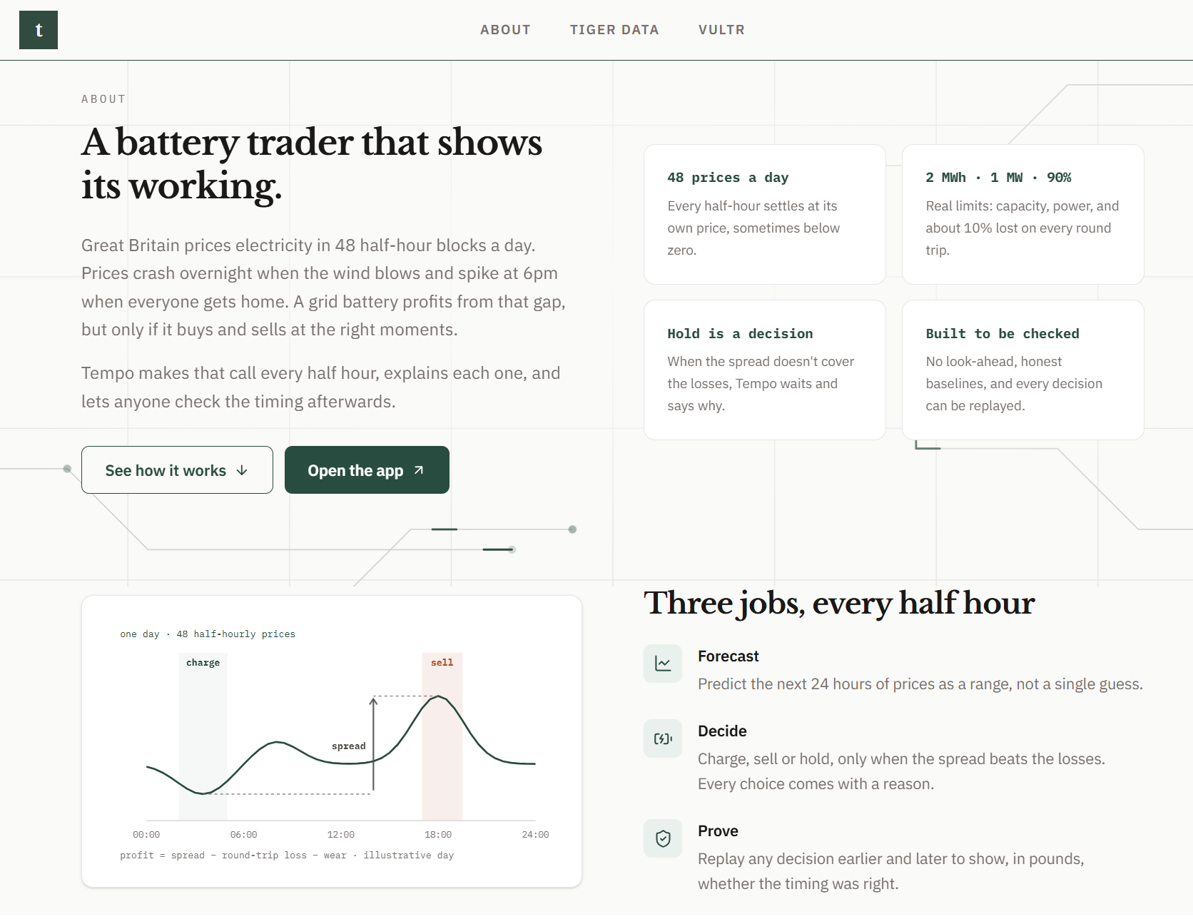
Electricity in Great Britain is priced every half hour. At 3am on a windy night, wind farms produce more than the country needs and the price collapses, sometimes below zero. At 6pm on a cold weekday, everyone gets home, switches on the oven and the heating, and the price spikes. A grid battery makes money in the gap between those two moments.

The theme was TIME, and this felt like the most literal version of it we could find. A battery doesn't really need to know what the price will be. It needs to know when to act. Charge an hour too early and you overpay. Sell an hour too late and the peak has gone.

We were also building for HRT's track, Best Use of Data for Predictions and Decision Making. The obvious hackathon project in that space is "a model that predicts whether a price goes up", usually reported as an accuracy number on a random train/test split. We wanted the opposite: a system that turns a forecast into a constrained decision, measures that decision in pounds on data it has never seen, and then checks whether the decision was made at the right time.

What it does

Tempo has three layers.

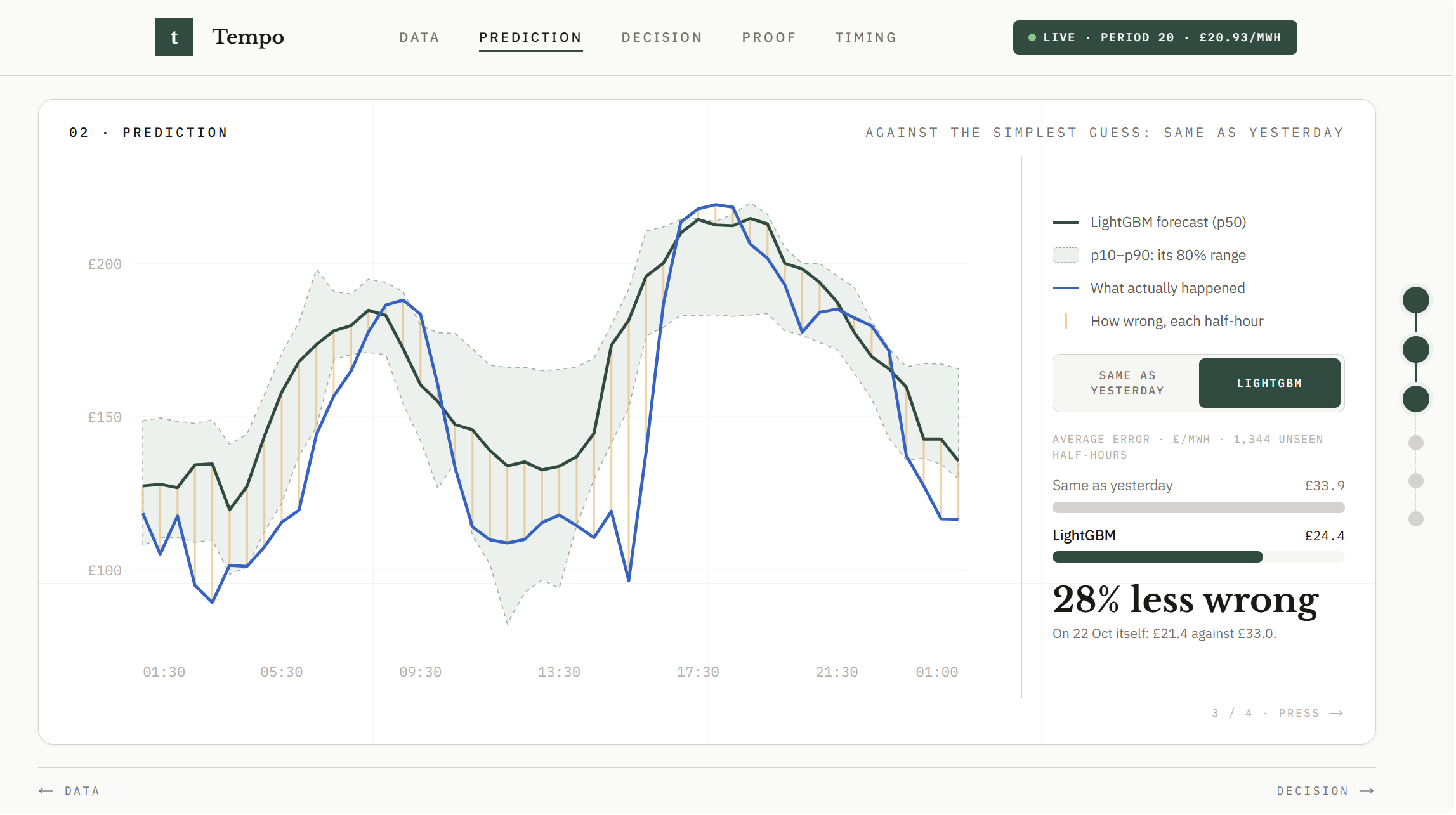
A live decision engine. Every half hour it pulls Elexon market data into Tiger Data, forecasts the next 48 prices as a $p_{10}/p_{50}/p_{90}$ band, and commits to charge, discharge or hold for each period, with a written reason on every row.
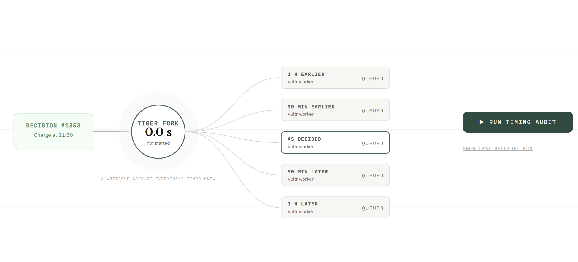
A timing audit. Click any decision and Tempo replays it one hour early, half an hour early, on time, half an hour late and one hour late, in parallel, and shows in pounds what rushing or hesitating would have cost.
An honesty panel. Results on weeks the model never saw, against honest baselines, as a share of what perfect knowledge of the future would have earned.

How we built it

Data: from Elexon to Tiger Data

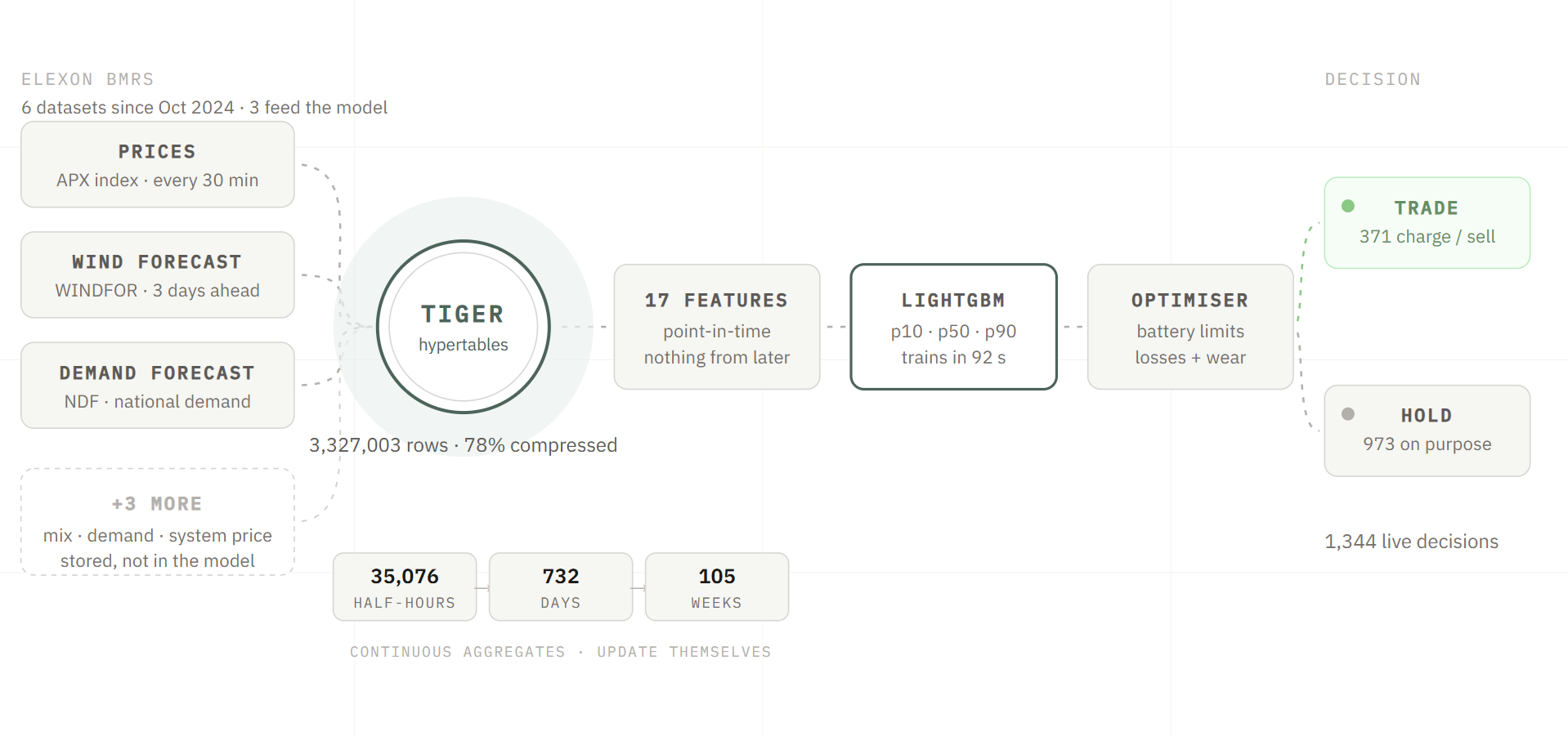
We pull six datasets from the Elexon Insights API (prices, wind forecast, demand forecast, outturn demand, generation mix and system prices) with a two-year backfill and a live poller. Everything lands in Tiger Data hypertables, rolled up by continuous aggregates into half-hourly, daily and weekly prices, with compression keeping two years of history inside the free tier.

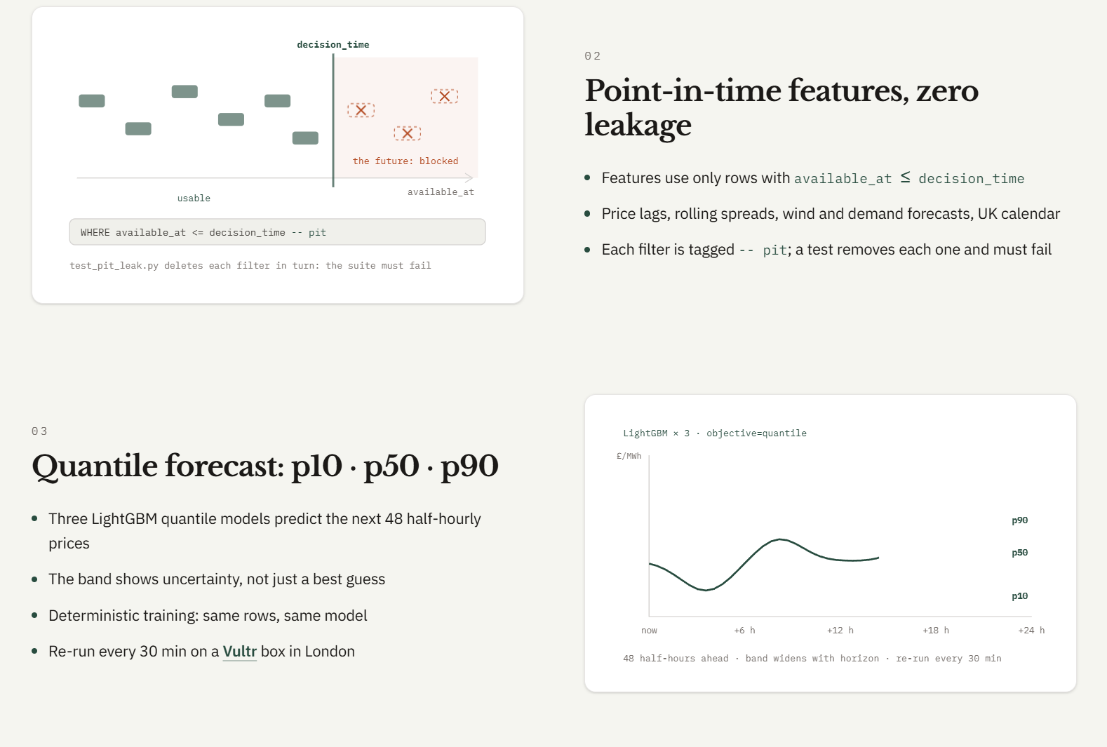
The most important design decision in the whole project was point-in-time stamping. Every row stores available_at, the moment Tempo could first have seen it. A feature for a decision at time $t$ is built only from

$$ \mathcal{D}(t) = \lbrace\ r : \texttt{available\textunderscore at}(r) \le t\ \rbrace. $$

The price series we use (APX Market Index Data) has no publish time, so we state one conservatively:

$$ \texttt{available\textunderscore at} = \texttt{start\textunderscore time} + 30\ \text{min} + 10\ \text{min}. $$

Every point-in-time filter in the SQL is tagged -- pit. A test deletes each one in turn, and the test suite has to fail every time. If it doesn't, the filter wasn't doing anything.

Forecast: quantile LightGBM

Three LightGBM models predict each of the next 48 half-hours, one per quantile $\alpha \in \lbrace 0.1, 0.5, 0.9 \rbrace$, each trained on the pinball loss

$$ L_\alpha(y, \hat y) = \max\big(\alpha (y - \hat y),\ (\alpha - 1)(y - \hat y)\big). $$

Quantile models are fitted independently, so their outputs can cross. We sort them per row so that $p_{10} \le p_{50} \le p_{90}$ always holds. We climbed the model ladder simplest first: a persistence baseline ("same price as yesterday") had to be beaten before LightGBM earned its place.

Decision: a cost-gated optimiser

The simulated battery holds $E = 2$ MWh, moves $P = 1$ MW, has round-trip efficiency $\eta = 0.9$, and costs $c = £20$ of wear per full cycle. Each half-hour period trades at most $e = P \times 0.5\ \text{h}$, and the efficiency loss is split evenly between charging and discharging:

$$ \text{SoC}_{t+1} = \begin{cases} \text{SoC}_t + e\sqrt{\eta} & \text{charge} \ \text{SoC}_t - e / \sqrt{\eta} & \text{discharge} \end{cases} \qquad 0 \le \text{SoC} \le E. $$

A buy/sell pair only makes money if the spread beats the efficiency loss and the wear, so Tempo trades only when

$$ \eta\ p_{\text{sell}} - p_{\text{buy}} > \eta \cdot \frac{c}{E}. $$

Otherwise it holds and logs why. On a flat day, doing nothing is the right decision, and a system that can't hold bleeds money.

We built two optimisers. The live one is a greedy rule that repeatedly pairs the cheapest buy period with the dearest later sell period. The second is a cvxpy linear program over the full 48-period horizon:

$$ \max_{c_t,\ d_t \ge 0}\ \sum_{t=1}^{48} 0.5\ p^{(50)}_t (d_t - c_t)\ -\ 0.5\ w \sum_{t=1}^{48} d_t $$

where $c_t$ and $d_t$ are charge and discharge power and $w = c/E$ is wear per MWh discharged, subject to the state-of-charge, power and efficiency constraints above.

Timing audit: Tiger forks and Vultr workers

When you click a decision, Tempo takes a Tiger Data zero-copy fork of the live database: a writable, copy-on-write copy frozen at that instant. It then sends five timelines, the same schedule shifted by $k \in \lbrace -2, -1, 0, +1, +2 \rbrace$ half-hours, to five pre-warmed Vultr workers in parallel. Each worker is a small FastAPI service that connects to the fork, replays the battery at actual prices and returns its profit. The audit reports

$$ \Delta_k = \text{PnL}(k) - \text{PnL}(0), $$

the cost of acting $k$ periods early or late. The same analysis runs automatically on every completed cycle as a self-grade: Tempo's timing counts as "within one period" when $\arg\max_k \text{PnL}(k) \in \lbrace -1, 0, +1 \rbrace$.

A separate Vultr box in London runs the poller, the live decider every 30 minutes, and the Streamlit dashboard.

Measuring it honestly

We ran a walk-forward backtest: 28 days of training, retrained for every 7-day test week, over 100 unseen weeks. Raw pounds swing wildly between calm and volatile weeks, so the headline metric is the share of perfect foresight captured:

$$ \text{score} = \frac{\sum_{w} \text{PnL}^{\text{Tempo}}_w}{\sum_{w} \text{PnL}^{\text{perfect}}_w}. $$

Strategy	Money made	% of perfect
Fixed rule (charge 1-5am, sell 5-7pm)	£29,265	33.1%
Persistence forecast + same optimiser	£46,798	52.9%
Tempo (LightGBM + greedy, live)	£58,711	66.4%
Tempo LP (LightGBM + LP)	£60,391	68.3%
Perfect foresight	£88,388	100%

The persistence row uses the same optimiser as Tempo, so the gap between them isolates the value of the model itself.

Stack: Python, Tiger Data (TimescaleDB), LightGBM, cvxpy, pandas, FastAPI, Streamlit, Vultr, and a Next.js presentation site.

Challenges we ran into

We designed the audit as one Tiger fork per timeline. When we ran it against the real service, the third fork was refused with 403 ENTITLEMENT_ERROR: a free Tiger project holds only two services at once, the live database plus one fork. Paying wouldn't have helped either, because the fast copy-on-write forks only exist on free services, and paid forks take 5 to 20 minutes. We redesigned the audit around one shared fork per click, with each timeline writing under its own run id, and wrote a test proving the result is identical to the penny.

Elexon's data has sharp edges. The Market Index price has no publish time, so we had to state an availability delay. Clock-change days have 46 or 50 settlement periods, not 48, so we key everything on UTC start time and never on "settlement day + period". One endpoint rejects windows longer than a day, and the N2EX price index is full of zero-volume, zero-price rows, so we use APX.

Lookahead is easy to introduce and hard to see. Interpolating an hourly wind forecast to 10:30 quietly uses the 11:00 forecast, which may not exist yet at decision time. We forward-fill instead. That's why we built the leak test that deletes each point-in-time filter and expects the test suite to fail.

Cold starts are too slow for a live click. A new Vultr instance took about 40 seconds to boot and 80 seconds to accept SSH. So the five workers run all day, built from one snapshot, and a click only has to find them through the Vultr API by tag. A simple lease-based scheduler keeps it to one job per worker and queues the rest.

We also had three people working on one schema. We split the work three ways: data, model and optimiser, and the audit plus the dashboard. To work in parallel, we froze the database schema and the interfaces between modules on day one and built against a synthetic dataset until the real data landed.

Accomplishments that we're proud of

It runs live rather than in a notebook. Tempo polls Elexon, forecasts and commits a decision every half hour from a Vultr box in London, writing to Tiger Data, with no laptop involved.
It beats honest baselines on unseen data. Over 100 weeks the model never saw, Tempo captured 66.4% of perfect foresight: 2× a fixed-hours rule, and 13.5 points above a persistence forecast running the same optimiser. It never lost money in a single week (worst week 31.2%).
The timing audit works end to end. One click takes a Tiger zero-copy fork in about 40 seconds and replays five timelines on five Vultr workers in parallel, and a test proves the result matches the in-process replay to the penny.
We can prove there's no lookahead. Every row carries the time it became available, and the leak test fails if any single point-in-time filter is removed.
Every decision explains itself. All 48 rows in every batch, trades and holds alike, carry a plain-English reason.
We published our weak spots. The honesty panel shows the overconfident uncertainty band and the regime result that went against our expectations, right next to the headline number.

What we learned

Point-in-time data is everything. A backtest is only as honest as its timestamps. The most valuable code we wrote was the boring line that says "only use rows available before now".

A decision is not a prediction. Physical constraints and costs turn a good forecast into a much harder problem, and a cost gate that can say "hold" was worth as much as a better model.

Start simple and stay there until the data says otherwise. The LP beat greedy by two points over 100 weeks. That wasn't enough to justify swapping the live system the night before the demo, so the LP sits on the honesty table as a row instead.

Show the bad numbers too. Our $p_{10}$ to $p_{90}$ band should contain about 80% of real prices. On 405 live forecasts it contains 40%, so the model is overconfident. Trades use $p_{50}$ only, so the band never changes a decision, and the dashboard says so plainly. We also expected forecasting to matter more in windy weeks, and it didn't. Both findings are on screen.

Test against the real service, not the brochure. The free-tier fork limit only showed up when we ran the real thing.

What's next for Tempo

Run the backtest on the Vultr fleet. The 100 test weeks are independent, so they can be split across the five workers. We want to add a /backtest endpoint next to /replay, prove the parallel run matches the sequential one row for row, and report a measured speed-up rather than an estimate.
Battery-size sweep. Re-run the backtest for 1, 2, 4 and 8 MWh to show how much a bigger battery is worth under the same strategy.
Fix the overconfident band. Recalibrate the $p_{10}$ to $p_{90}$ interval so it really contains about 80% of prices, then let the uncertainty shape decisions: the LP's conservative mode already prices buys at $p_{90}$ and sells at $p_{10}$, ready to switch on once the band can be trusted.
Promote the LP. With more live weeks behind it, switch the decider to the LP if it keeps its lead. It's one flag away (--optimiser lp).
One fork per timeline. On a Tiger account with a higher service limit, the original five-fork layout is already in the code behind one setting (TEMPO_AUDIT_FORKS=per_shift).