-

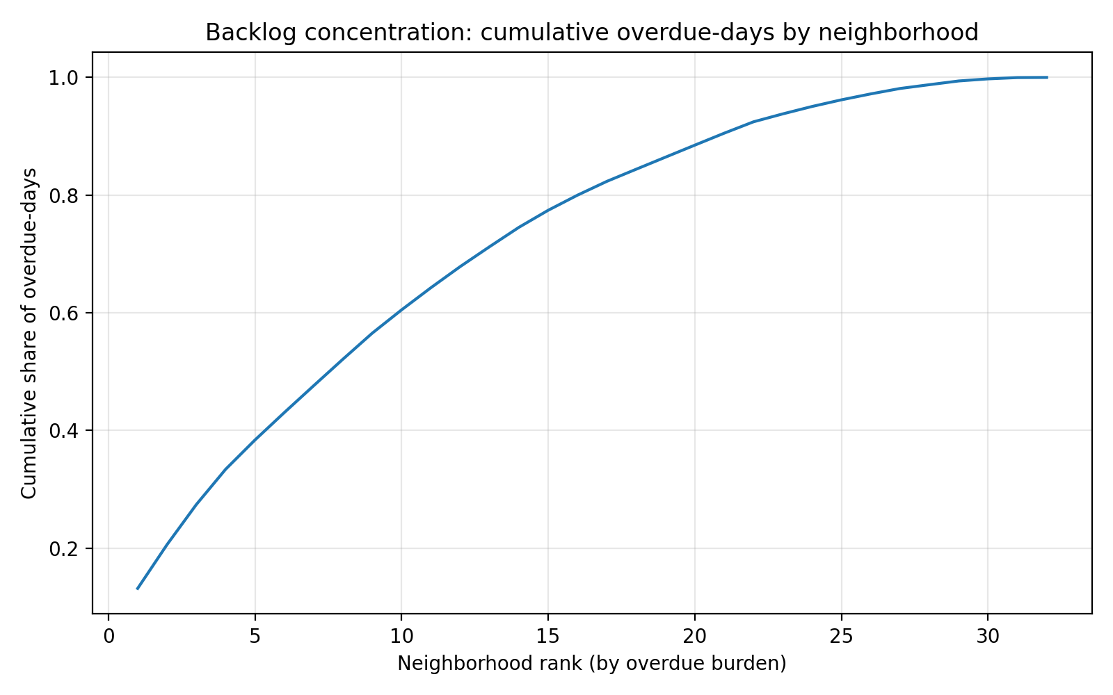
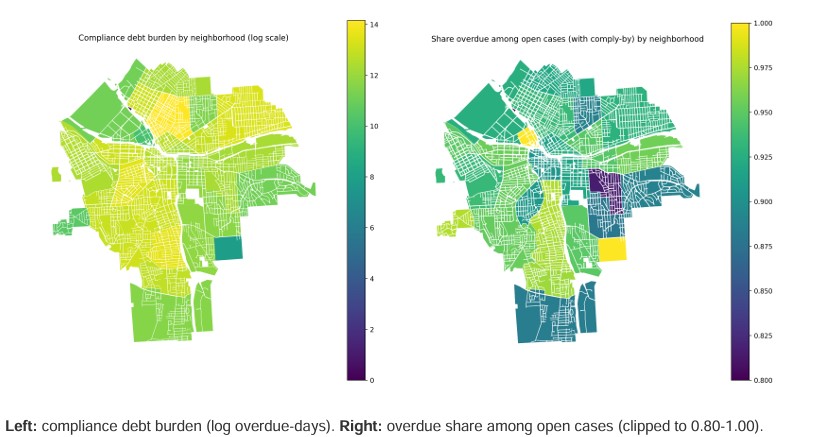
Interpretation: the first 10 neighborhoods account for about 60% of all overdue-days.
-

Neighborhood choropleths are built by dissolving parcel polygons and aggregating parcel-linked code records.
-

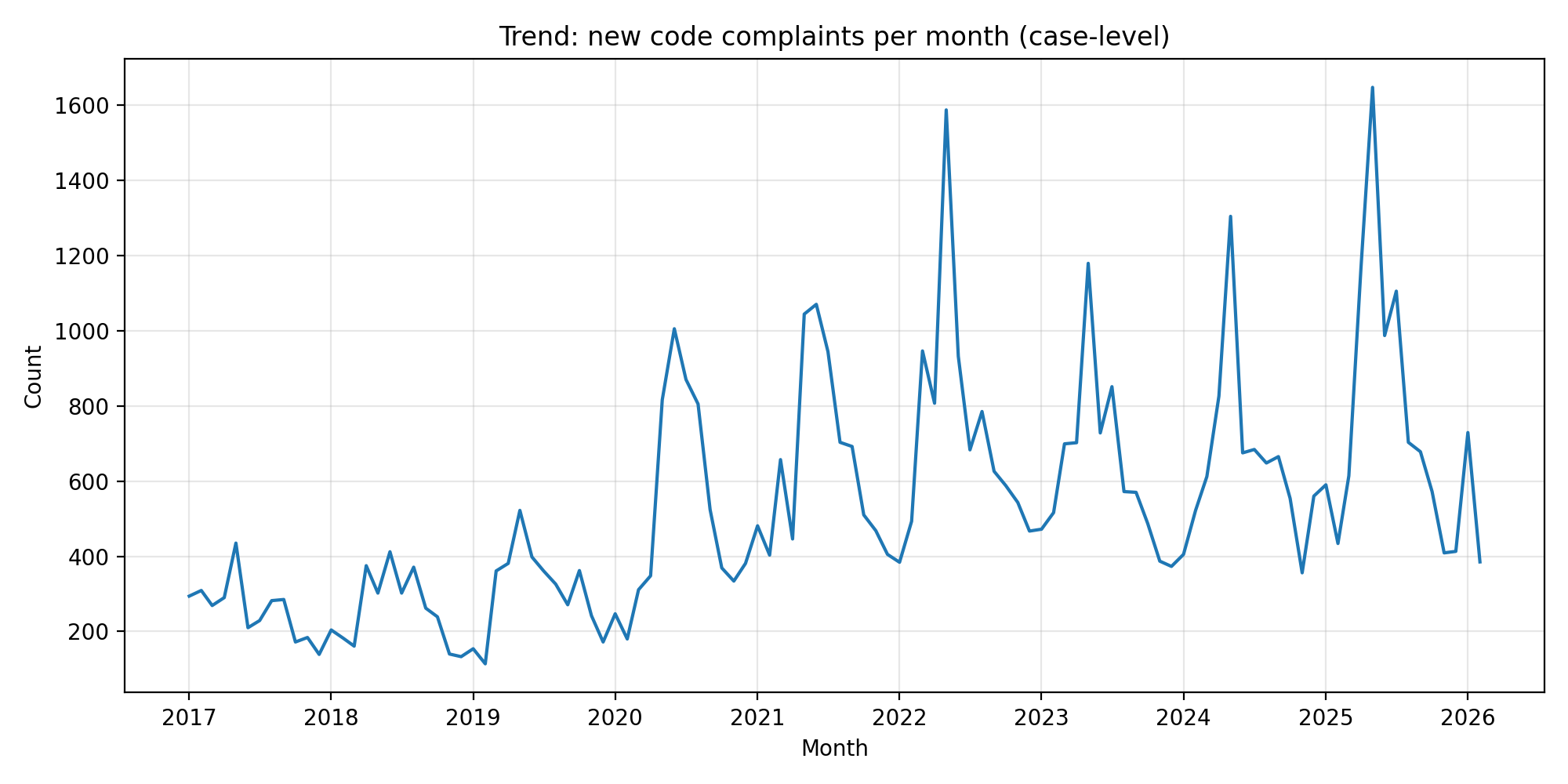
new complaint/case inflow over time
-
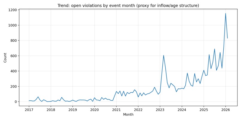
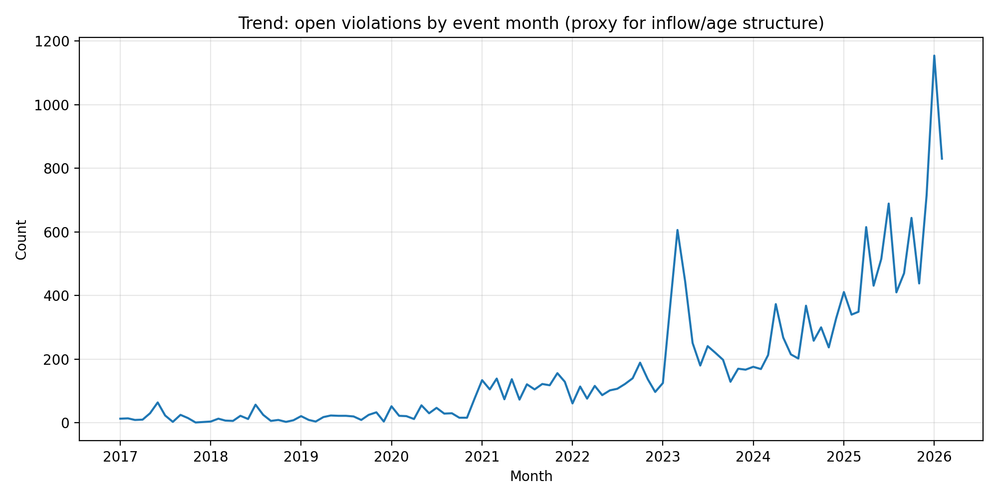
event-month distribution of currently-open violations
-
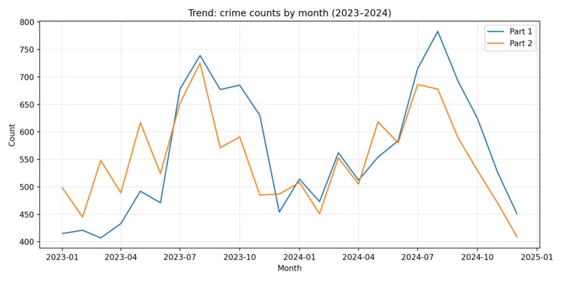
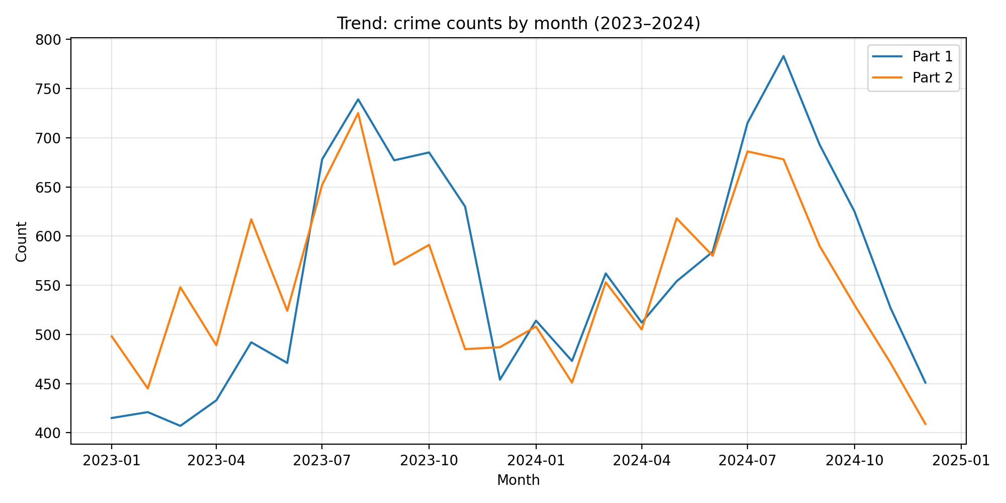
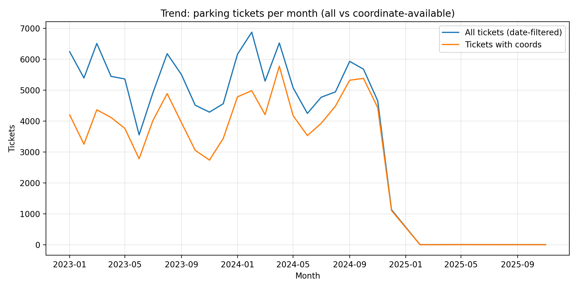
Crime trends use 2023-2024 (avoids partial 2025). Parking is shown as all tickets vs coordinate-available subset used for spatial features.
-
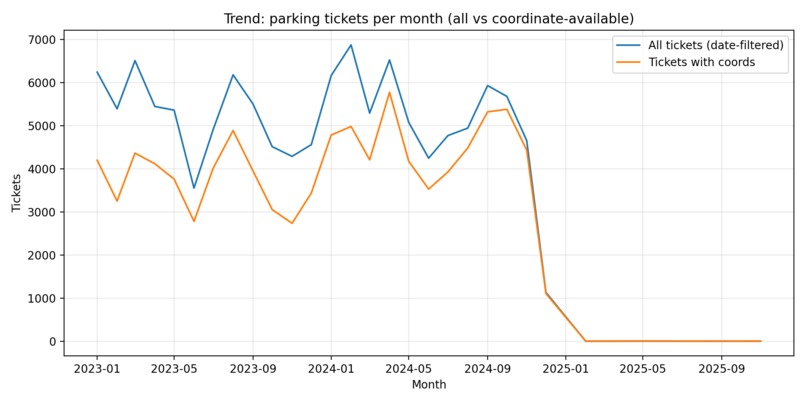
Crime trends use 2023-2024 (avoids partial 2025). Parking is shown as all tickets vs coordinate-available subset used for spatial features.
-

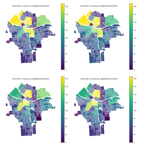
Maps use shared color scales (vmax capped at the 95th percentile across both years) for comparability.
Inspiration
City services like code enforcement operate under a hard constraint: inspection capacity is limited, but the “need” is not. When we explored Syracuse’s open municipal datasets, one pattern immediately stood out that many open code cases were already past their comply-by dates. That raised a simple question with real operational value:
If the backlog (“compliance debt”) is so large, where is it concentrated, and how can we visualize actionable priorities?
We built this project to make that answer obvious in a single visual story: debt hotspots, pressure signals (crime/parking), and a validated risk surface for what might happen next.
What it does
Cuse-RiskLens is a visualization-first risk mapping system that:
- Quantifies compliance debt: how overdue open code cases are relative to comply-by dates.
- Shows where the backlog concentrates (inequality / concentration curve + choropleths).
- Compares crime and parking hotspots across 2023 vs 2024 using shared color scales for honest year-to-year comparison.
- Produces an actionable parcel risk ranking (next-month risk) and a validated neighborhood risk surface.
Our core “decision” visualization is Precision@K: if a team can inspect only the top (K\%) highest-risk parcels, how many true next-month cases can they catch compared to random selection?
How we built it
Data sources (provided datasets only)
We used only the City of Syracuse datasets provided for Track 3:
- Parcel Map (Q1 2024) for parcel geometry, neighborhood/tract context, and parcel attributes.
- Code Violations (2017–present) as the enforcement signal (including comply-by dates and open/closed status).
- Crime datasets (2023–2025; our comparisons focus on complete years 2023–2024).
- Parking Violations (2023–present; maps use the coordinate-available subset).
Pipeline (reproducible)
We implemented a reproducible notebook pipeline:
- Load + clean
- Standardize column names, parse dates, normalize IDs.
- Filter implausible coordinates/timestamps (e.g., future-date artifacts).
- Integrate
- Join code violations to parcels primarily using SBL (high match rate).
- Dissolve parcel polygons into neighborhood boundaries for consistent mapping.
- Feature engineering
- Monthly aggregation for crime/parking pressure signals.
- Rolling windows for recent pressure: (30/90)-day and (3/6)-month rollups (depending on layer).
- Visualization-first analysis
- Log-scaled burden maps for heavy-tailed distributions.
- Shared-scale side-by-side maps (2023 vs 2024) for crime and parking.
- Validated prediction
- Train a LightGBM model (hygiene version removing ID-like fields).
- Time-based backtesting (train (\le T), validate at (T)) with operational metrics.
Model objective
We framed prediction as a ranking problem:
- Target: does a parcel receive a new code complaint in the next month?
- Evaluate ranking quality using:
- PR-AUC (appropriate for rare events)
- Precision@K (directly interpretable for inspection capacity)
Challenges we ran into
- Messy timestamps and partial-year coverage
Some datasets contained out-of-range timestamps (e.g., far-future values) or partial-year exports. We added strict plausibility filters and limited year-over-year comparisons to complete years. - Coordinate availability differences
Parking data had a substantial fraction of rows without coordinates. We separated “all tickets” trends from “coordinate-available tickets” trends to avoid misleading conclusions. - Fair map comparison
Choropleths can be deceptive if each year uses a different color scale. We enforced shared scales across years (and used robust caps when needed) to make comparisons honest. - Avoiding “leaky” predictors
GIS exports often include internal identifiers (e.g.,objectid). We implemented a hygiene model that removes ID-like fields to keep the story credible to judges.
Accomplishments that we're proud of
- Built a visualization-first story where each figure has one clear takeaway.
- Quantified and mapped compliance debt in a way that is immediately actionable.
- Produced shared-scale year-over-year hotspot maps (crime and parking) that support honest comparison.
- Delivered a validated risk surface and Precision@K actionability framing and translating ML performance into operational decisions.
What we learned
- Visualization quality isn’t just aesthetics but it is scale choices, comparability, and honest encoding determine whether a map misleads or informs.
- For rare-event civic problems, PR-AUC + Precision@K communicates value better than accuracy.
- “Small data issues” (timestamps, missing coordinates, ID fields) can dominate outcomes unless handled early.
- A strong civic analytics project needs a spine (parcels/neighborhoods) that all signals can map onto.
What's next for Cuse-RiskLens
- Add Vacant and Unfit property datasets to refine severity tiers (e.g., distinguishing “overdue but low risk” vs “overdue + high hazard”).
- Improve spatial granularity with grid/hex hotspots (in addition to neighborhood aggregation) for corridor-level targeting.
- Add simple calibration (e.g., isotonic/Platt) so risk scores can be interpreted more like probabilities where appropriate.
- Build an interactive dashboard layer for stakeholders (while keeping the offline, reproducible pipeline intact).
Metrics we highlight (for judges)
If a neighborhood’s baseline next-month case rate is (p), and our top-(K\%) selection has precision (P@K), then the operational “lift” is:
$$ \text{Lift@K} = \frac{P@K}{p} $$
This converts model performance into “how many more true cases we catch per inspection,” which is the real operational goal.
Built With
- data.syr.gov
- geopandas
- lightgbm
- matplotlib
- pandas
- pyarrow
- python
- scikit-learn
- shapely
- streamlit

Log in or sign up for Devpost to join the conversation.