-
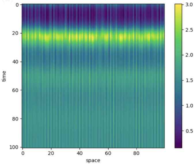
CML models for Bx.
-
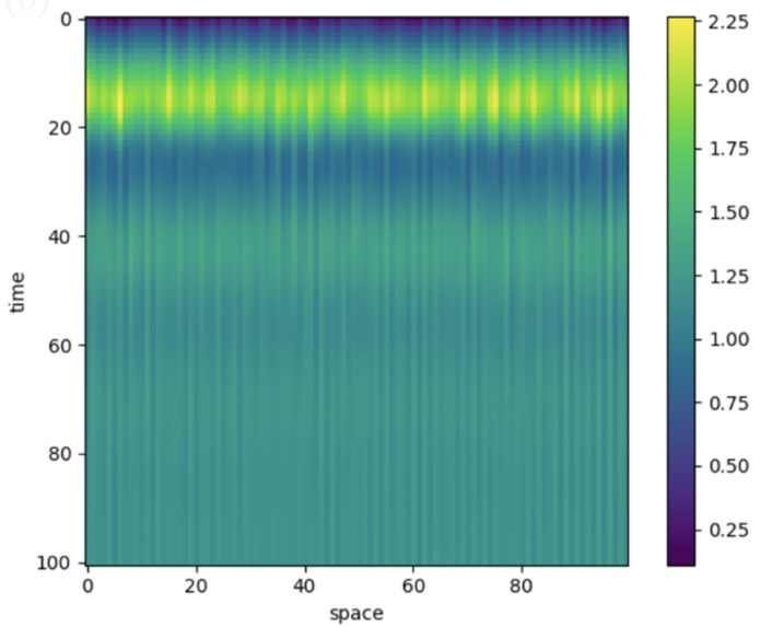
CML model for N.


Inspiration
Ecological systems look chaotic on the surface, but underneath, they are governed by simple local interactions: how nutrients move, how plants grow, and how matter is recycled. I was fascinated by the idea that complex ecosystem-level patterns can emerge from a few mathematical rules operating at the local scale.
This project was inspired by a single question:
How do microscopic nutrient exchanges give rise to macroscopic ecosystem stability or instability?
What it does
This project simulates how nutrients and plant biomass evolve over time and space in a minimal ecosystem.
It models:
- Nutrient supply, uptake, loss, and recycling
- Growth and decay of primary producer biomass
- Spatial interactions between neighboring ecosystem patches
The ecosystem is described by a coupled dynamical system:
$$ \frac{dN}{dt} = S - eN - cNB + r l B $$
$$ \frac{dB}{dt} = cNB - lB $$
where
(N) is the limiting nutrient,
(B) is plant biomass,
(S) is nutrient supply,
(e) is nutrient loss (efflux),
(c) is uptake rate,
(l) is biomass loss,
and (r) is the recycling rate.
To capture spatial dynamics, these equations are extended using a Coupled-Map Lattice (CML).
How I built it
I implemented two computational models in Python:
1. Single-cell ecosystem model
I implemented the coupled ODEs to simulate nutrient–biomass dynamics in one isolated ecosystem. This revealed oscillations, collapse, and equilibrium behavior depending on biological parameters.
2. Spatial ecosystem with CML
I placed the same model on a one-dimensional lattice. Each cell follows the same equations but exchanges nutrients and biomass with its left and right neighbors:
$$ X_i^{t+1} = (1-\varepsilon) f(X_i^t) + \frac{\varepsilon}{2} \left[f(X_{i-1}^t) + f(X_{i+1}^t)\right] $$
This introduces spatial flow, allowing waves, patches, and asynchronous peaks to emerge.
I performed parameter sweeps over:
- Efflux rate
- Recycling rate
- Nutrient supply
- Uptake rate
and visualized results using time-series plots, parameter-space plots, and spatiotemporal heatmaps.
Challenges I ran into
Finding biologically realistic and numerically stable parameter ranges was difficult. Many values caused the system to explode or collapse.
The CML model also added complexity: small changes in coupling strength or initial conditions produced very different spatial patterns, making debugging and interpretation harder than in the single-cell model.
Accomplishments that I'm proud of
- Built two consistent ecosystem models (ODE + CML)
- Identified dominant biological parameters using parameter-space analysis
- Visualized spatiotemporal chaos and spatial propagation
- Demonstrated how simple local rules generate complex global behavior
What I learned
I learned how nonlinear dynamical systems and spatial coupling can explain real ecological complexity. I gained experience translating biological assumptions into equations, analyzing stability, and interpreting chaotic simulations.
These skills directly transfer to AI, scientific computing, and complex systems modeling.
What's next for Spatial–Temporal Ecosystem Simulation with CML
Next, I want to extend this system to:
- 2D lattices for realistic landscapes
- Multiple species (e.g., predators and consumers)
- Stochastic noise to simulate climate variability
- GPU-accelerated simulations for large-scale ecosystems
This would transform the model into a powerful sandbox for studying ecosystem resilience, collapse, and recovery.

Log in or sign up for Devpost to join the conversation.