IEMS: an AI energy copilot for microgrids, running entirely on one NVIDIA GB10

IEMS (Intelligent Energy Management System) watches a real home microgrid second by second. It works out which appliances are running from the panel-level power alone, forecasts the next 24 hours of power, appliance use and battery charge, and turns those forecasts into plain advice such as "run the dishwasher at 1 PM, when the panels cover it" or "hold the battery, a wind alert is up." Every model is trained, served and retrained on a single ASUS Ascent GX10 (NVIDIA GB10 Grace Blackwell, 128 GB unified memory). It needs no cloud inference and no per-appliance meters, and it keeps running if the internet goes down.

Inspiration

Our test site is a working microgrid: a house in Los Gatos, California, with rooftop solar, a home battery, a backup generator and an eGauge meter on its sub-panels. Its owner, Dr. Pat Mantey, runs it through California's wildfire season. In that season PG&E can cut power pre-emptively during Public Safety Power Shutoffs, and the question changes from "what does energy cost?" to "what gets the stored energy?"

The meter shows three panel totals (HVAC, water, kitchen), not the twenty-plus appliances behind them. An operator sees Panel 3: 2.4 kW and has to guess whether that is the oven, the dryer or a fridge compressor. Per-appliance meters are expensive and invasive. They also don't exist in the remote and island microgrids where this question matters most.

So we asked whether a single box sitting next to the panel could:

see what each appliance is doing, from aggregate power alone (non-intrusive load monitoring, NILM),
anticipate the next day's demand, solar and battery state, and
advise, with reasons an operator can check,

with everything running locally on hardware a site could own. The GX10, with a Blackwell GPU and 128 GB of unified memory in a small desktop box, made that a realistic hackathon goal.

What it does

Tab	What the operator gets
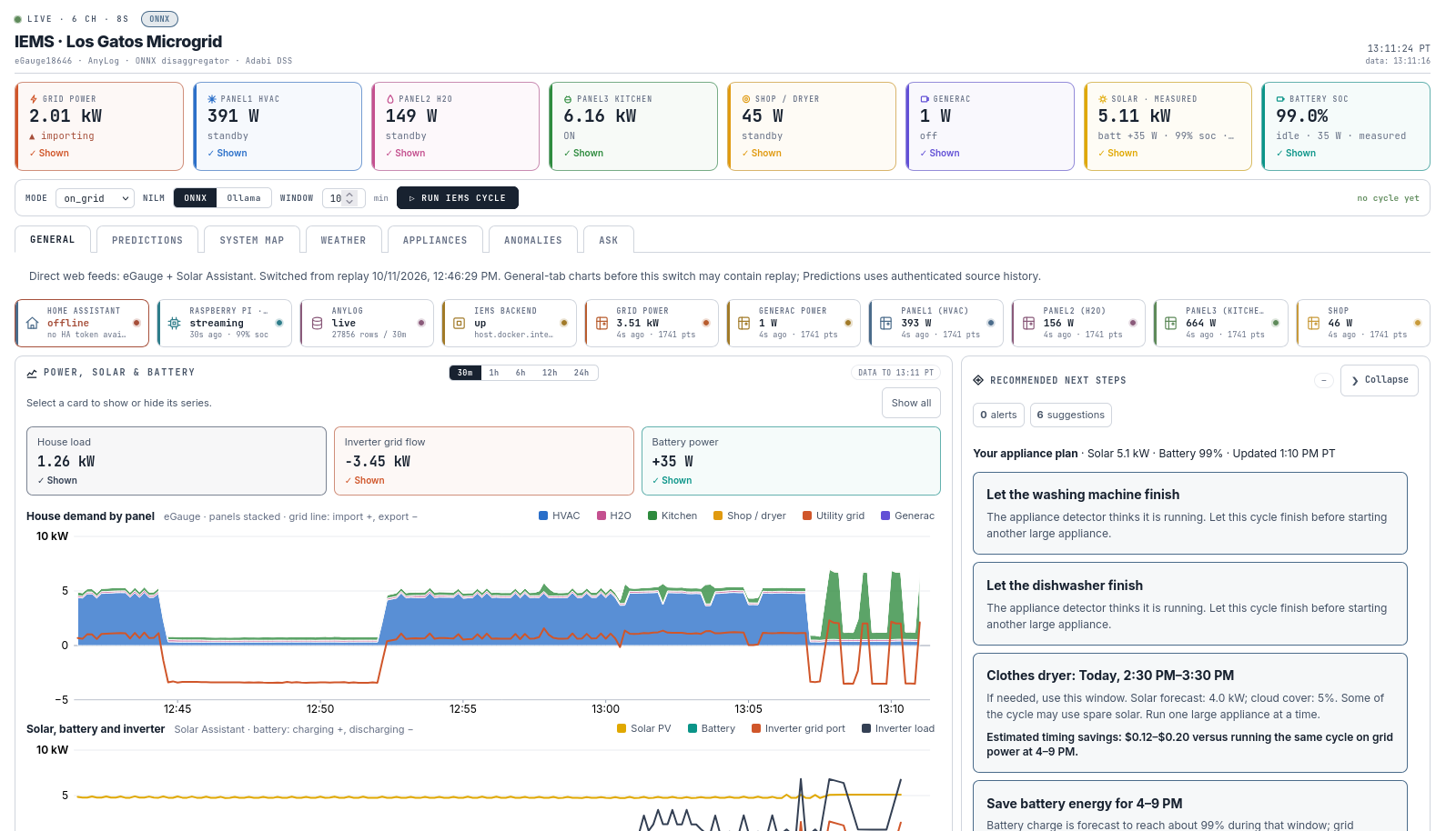
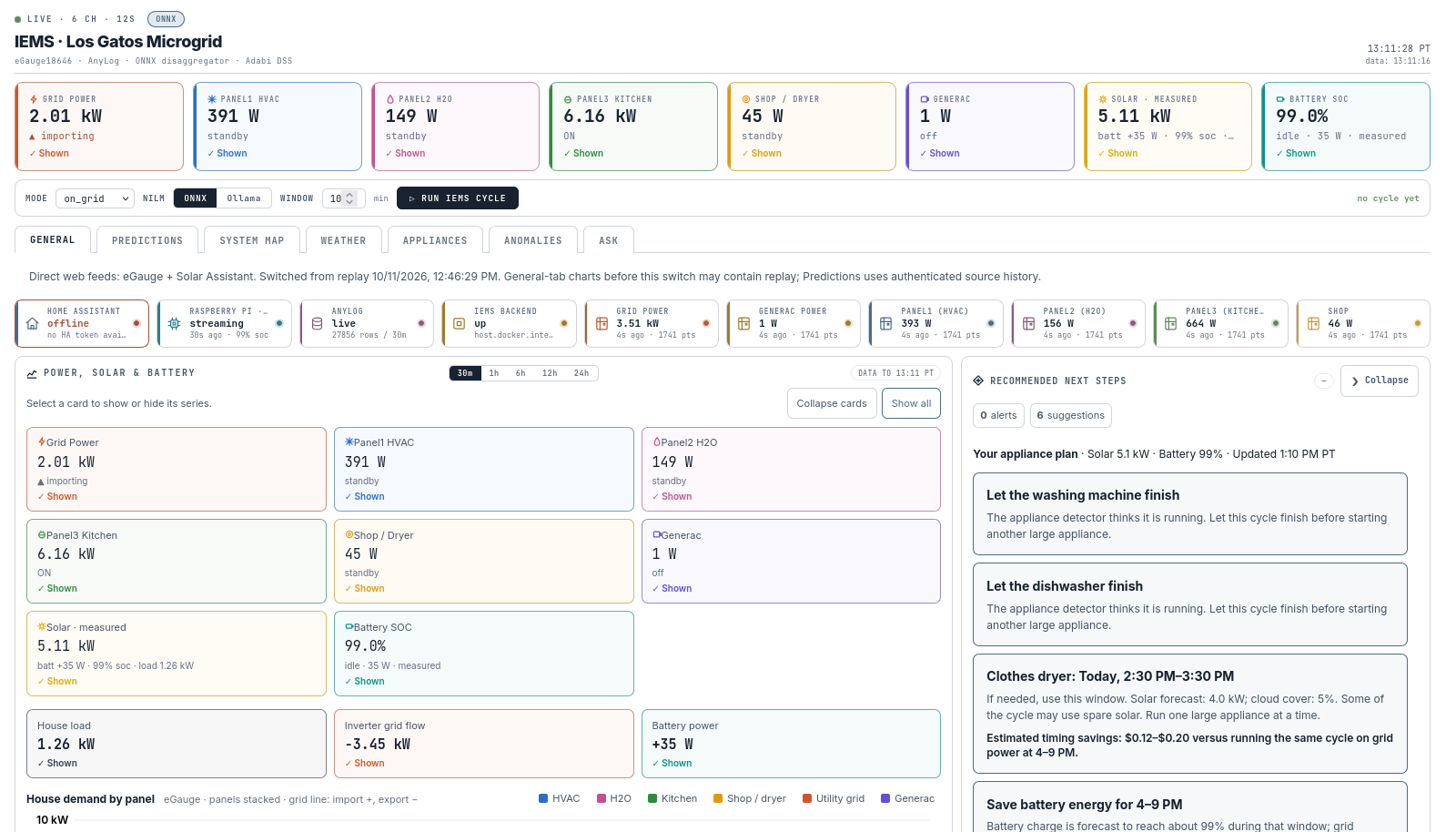
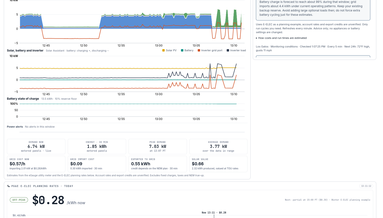
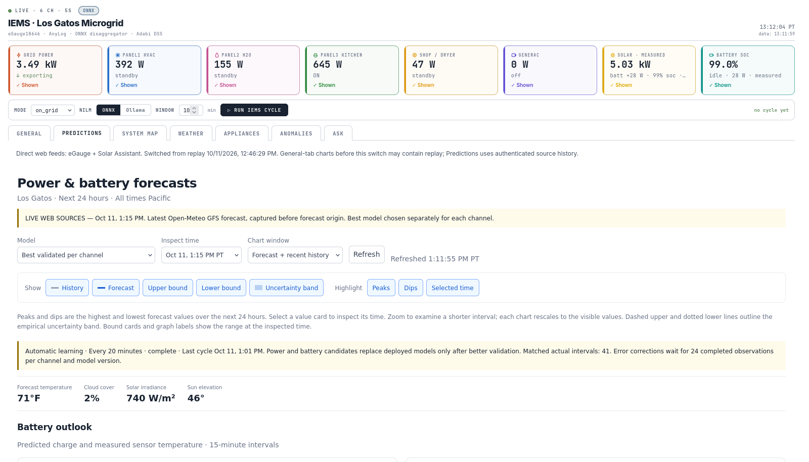
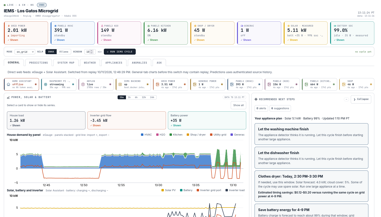
General	Live power cards for every panel, the grid, solar, battery and generator. Source freshness, the house demand chart, and "your appliance plan" advice cards.
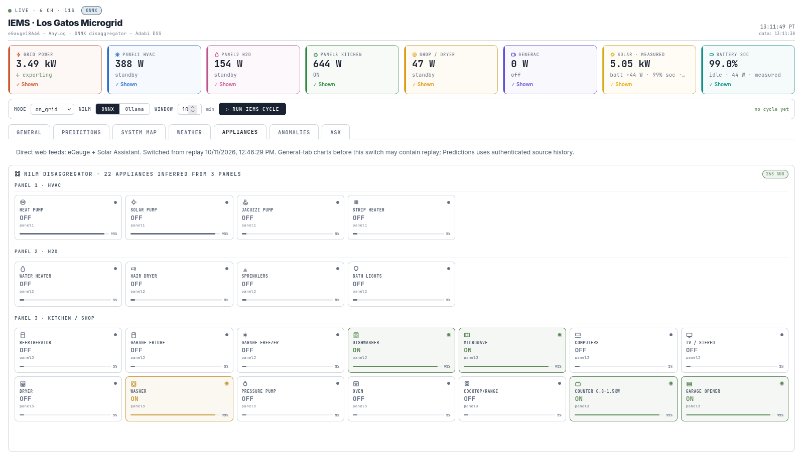
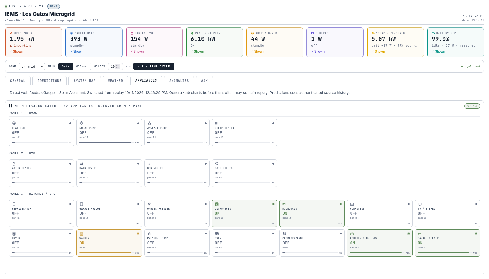
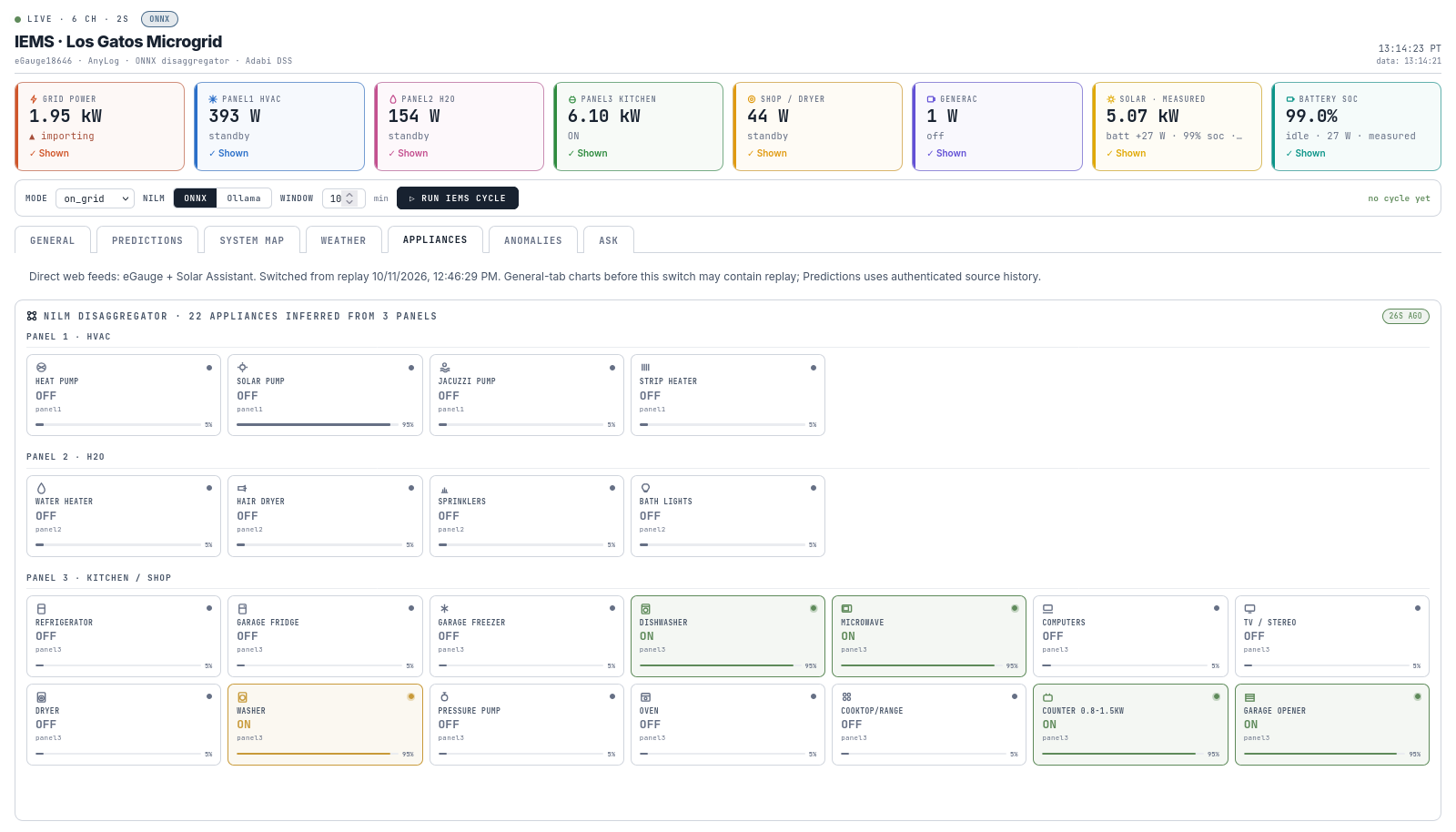
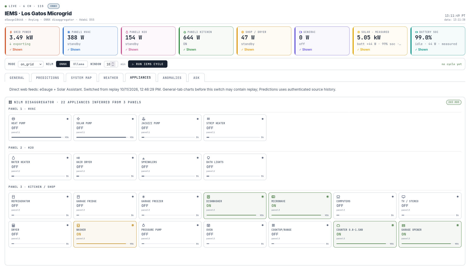
Appliances	Live ON/OFF state for 22 appliances across 3 panels, decided by our fine-tuned Nemotron 3.5 Lightning, with a per-appliance BiLSTM fallback.
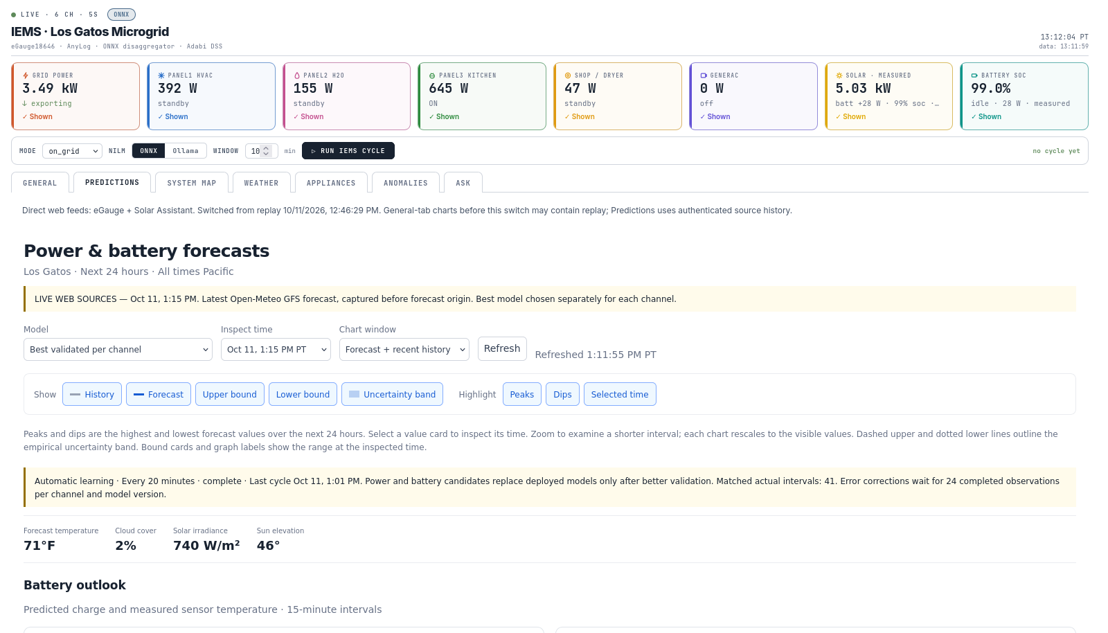
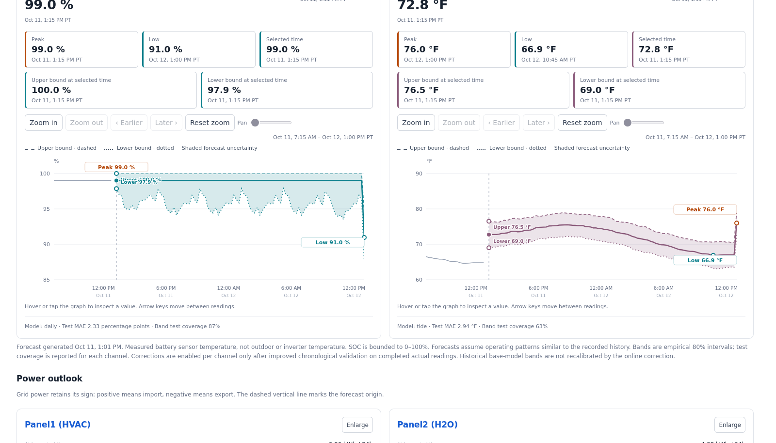
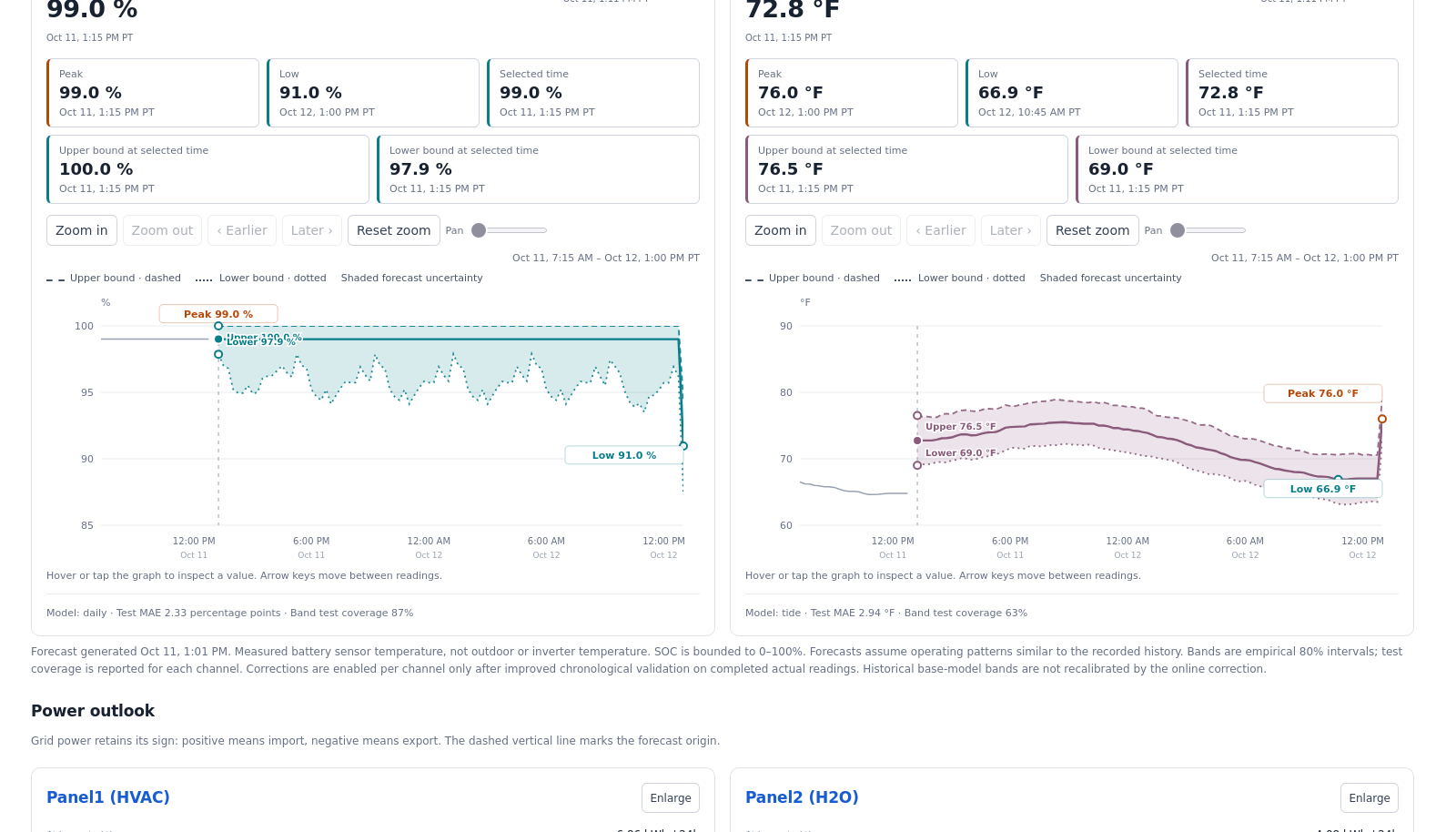
Predictions	24-hour forecasts in 15-minute steps for each panel, the grid, the shop, the generator and solar PV, plus the battery's charge and temperature. Each forecast has calibrated uncertainty bands.
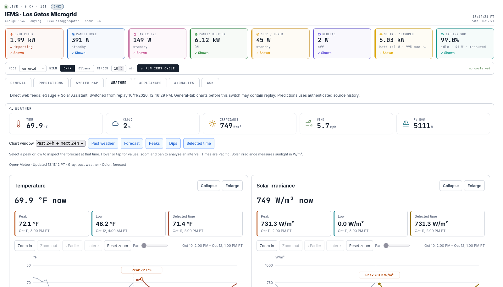
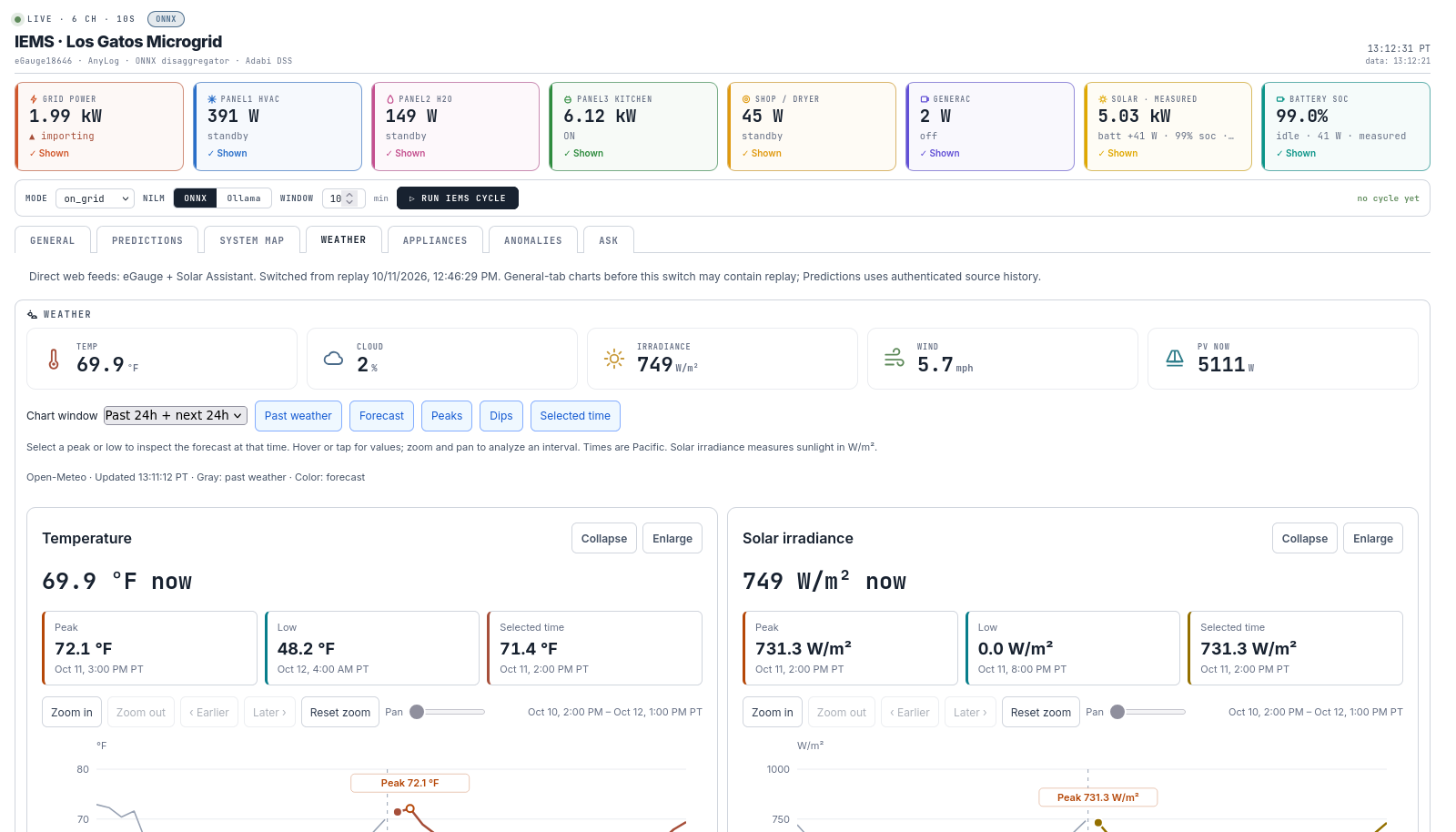
Weather	Temperature and solar irradiance, history and forecast. Feeds the readiness monitor (NWS alerts, PG&E outage and PSPS feeds).
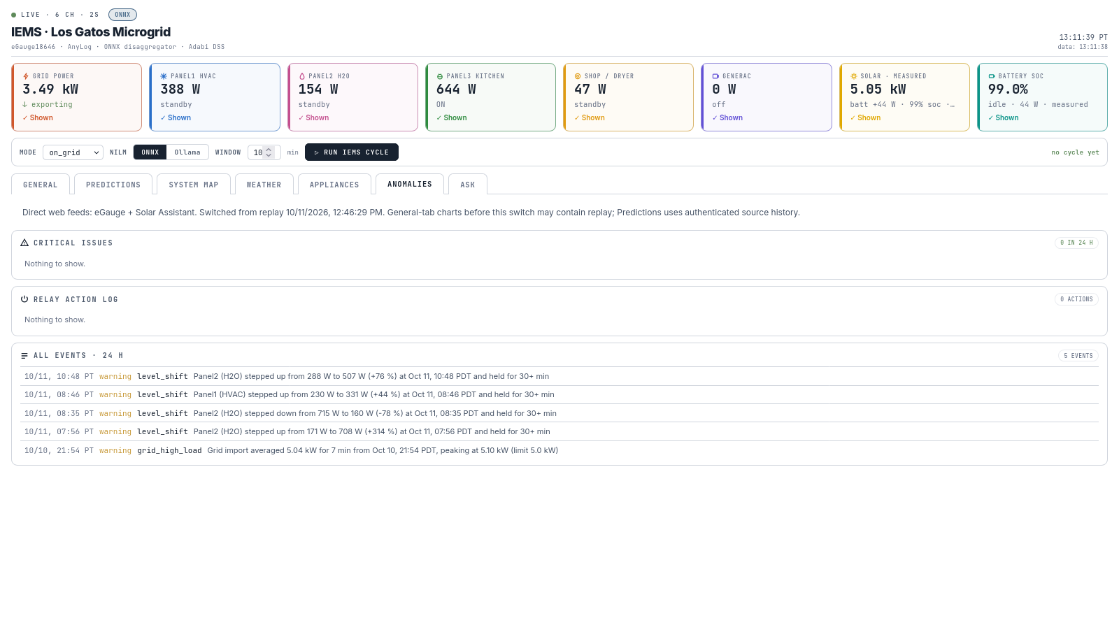
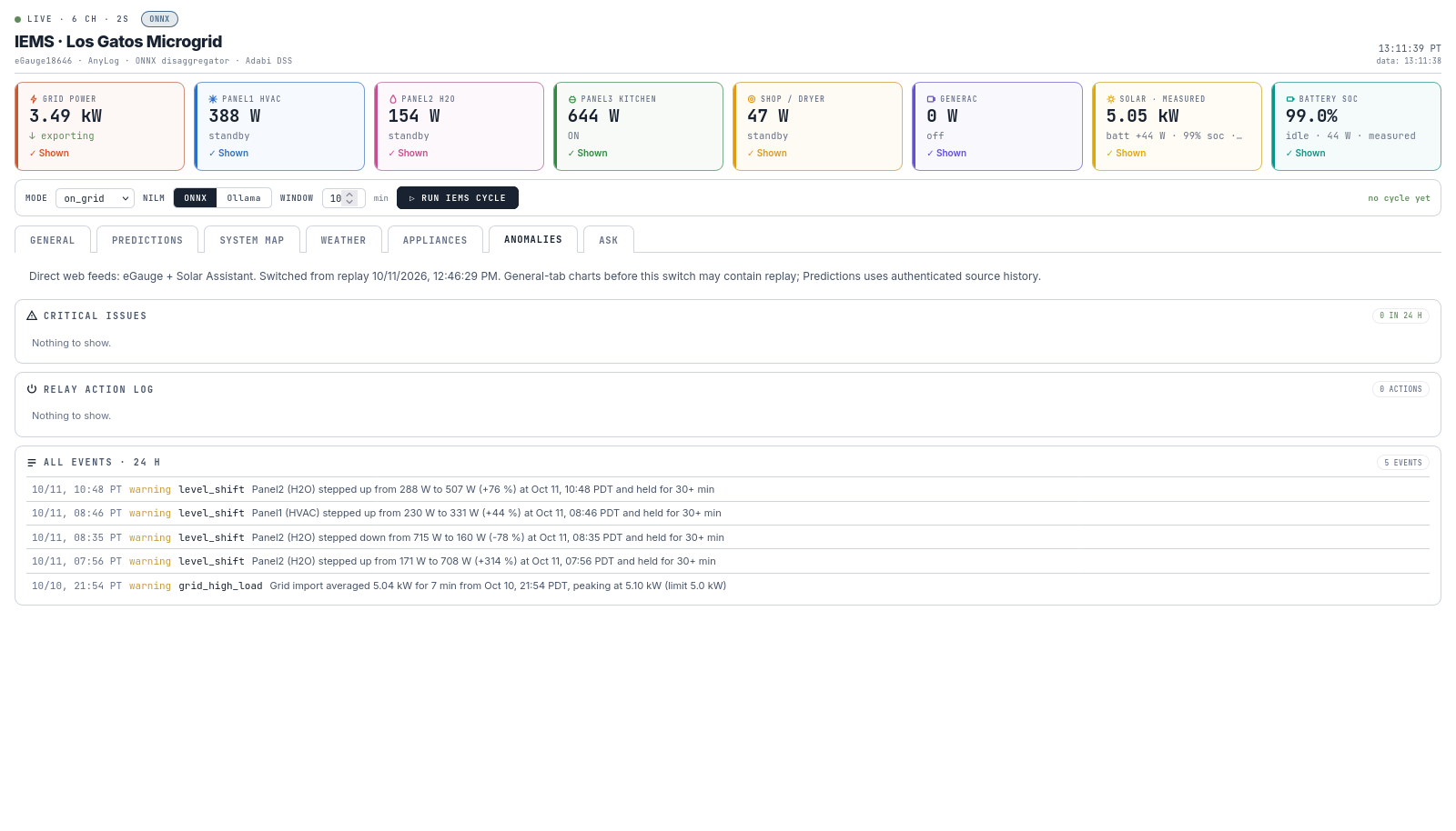
Anomalies	Critical issues, relay actions and an event log of unusual panel behaviour.
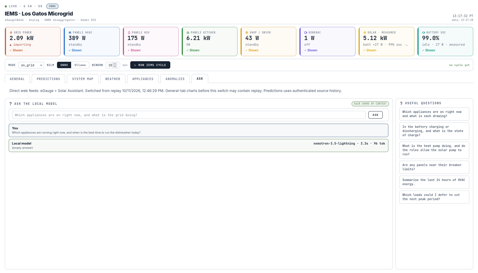
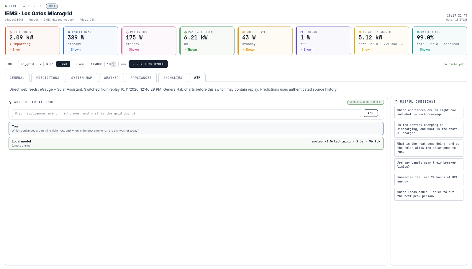
Ask	A chat assistant grounded in the live telemetry, answered by Nemotron 3.5 Lightning running locally in Ollama.
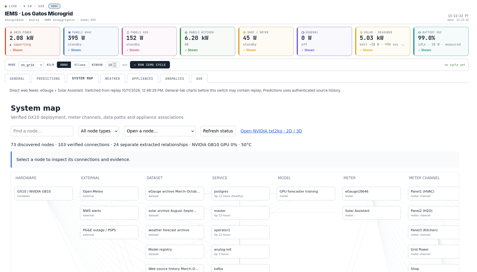
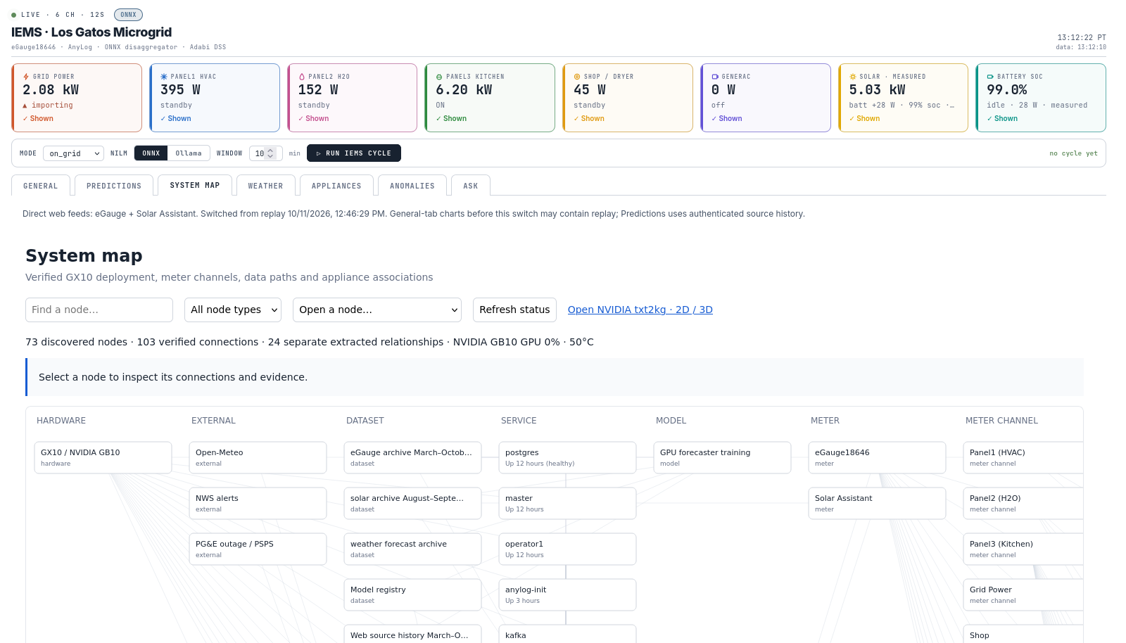
System map	A verified graph of the whole deployment: hardware, containers, data paths, meter channels and models. Built with NVIDIA txt2kg and ArangoDB.
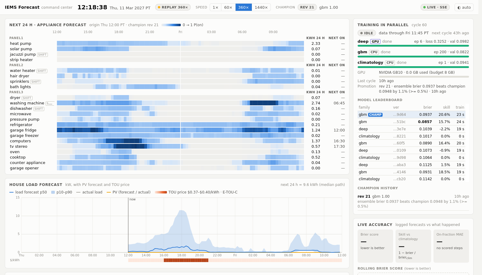
Appliance forecaster	A per-appliance, 24-hour forecast of the chance each appliance is on. It retrains continuously and hot-swaps the winning model.

The decision layer (smart_dss.py) schedules optional heavy loads (dishwasher, washer, dryer) into the cheapest feasible windows. The readiness monitor switches to prepare mode when outage risk rises. Every recommendation is advisory: IEMS never changes inverter, battery or relay settings on its own.

How we built it

The data path

 eGauge (1 s, 16 channels) ─┐
 Solar Assistant (PV, battery, SOC) ─┤──▶ Kafka ──▶ AnyLog edge data fabric ──▶ PostgreSQL
 Open-Meteo, NWS, PG&E ─┘                      │
                                               ▼
                          GB10: NILM + forecasting + DSS ──▶ dashboards + Ask

History: 30,734,135 deduplicated eGauge rows (March 6 to October 9, 2026, all 16 channels) and 976,788 Solar Assistant records.
Live readings: authenticated, read-only web collectors poll eGauge every 10 s and Solar Assistant every 30 s. A replay producer, which streams the archive with live timestamps, stays available as an opt-in demo mode.
Data fabric: AnyLog (arm64 image) runs as master and operator nodes. It ingests from Kafka and stores in PostgreSQL. The dashboard queries it directly.
Compute: everything runs in Docker on the GX10. The GPU is shared by training, serving (llama.cpp, vLLM, Ollama) and the forecasters.

Model 1: physics labeller (labels without per-appliance meters)

Without per-appliance meters there is no ground truth, so we wrote down the physics instead. physical_labeler_v2.py labels every timestamp of the history using rules like these:

a 2–4.3 kW water-heater element cannot be on while the whole H2O panel draws under 1.6 kW;
the solar circulation pump is off when the sun is below the horizon;
a dishwasher in any active phase lifts the panel's oscillation component;
refrigeration compressor cycles are separated from the other loads.

Crucially, the labeller abstains (NaN) wherever physics can't decide, and attaches a confidence weight $w\in[0,1]$ to every label it does give. We relabelled the full history this way, 1,956,739 timestamps.

Model 2: per-panel BiLSTM (the teacher)

Each panel gets its own network. The input is a window $X\in\mathbb{R}^{100\times18}$ of 18 features:

the panel's own power and the other panels;
grid, shop, leg currents and voltage;
time of day as $(\sin,\cos)$;
solar elevation, clear-sky irradiance and measured PV.

Two bidirectional LSTM layers (32 then 16 units per direction) feed a small MLP per appliance. The 14-appliance kitchen panel uses a convolutional stem with a separate BiLSTM branch per appliance, so the fridge's slow cycling and the microwave's bursts don't compete for the same parameters.

Training is rolling walk-forward, so every reported metric comes from data the model had never seen:

split the history into $K=4$ chronological folds;
for stage $k$, train on folds $0..k-1$ (warm-started), then predict fold $k$ before training on it;
pseudo-label only the windows where the physics labeller abstained, then add fold $k$ to the training pool.

Appliances are heavily imbalanced (a hair dryer is on for minutes a day), so the loss is a masked, confidence-weighted BCE with $\text{pos_weight}$ up to 200. For the most extreme heads it switches to focal loss:

$$ \mathcal{L}_{\text{focal}} = -\alpha\,(1-p_t)^{\gamma}\log p_t,\qquad \gamma=2,\ \alpha=0.25 . $$

Decision thresholds are calibrated on the last fold. The models are exported to ONNX, then gated with power and mutual-exclusion rules. We retrained all three panels on the GB10 over the relabelled history. For example, the heat pump reaches F1 0.93 on the last unseen fold.

Model 3: Nemotron 3.5 Lightning as the live NILM engine

We wanted the appliance engine to be a model that can also explain itself and grow new skills. So we distilled the gated BiLSTM into NVIDIA Nemotron 3.5 Lightning 30B-A3B, a hybrid Mamba-2 / mixture-of-experts LLM with about 3B parameters active per token.

Prompt and answer contract. Each 10-minute panel window becomes a compact text prompt:

the panel's power at every second sample (50 values);
its mean, median, extremes and number of on/off edges over 100 W;
the other panels, grid, leg currents and voltage;
sun elevation and PV;
the list of appliances to decide.

The model answers one line per appliance, name=ON or name=OFF. Reasoning is turned off, so the answer is the whole reply. The same Python module builds the prompt in training and at inference, so the text is identical byte for byte.

LoRA fine-tuning with NVIDIA NeMo AutoModel (single-GPU recipe, CI-tested on the GB10, BF16):

$$ W = W_0 + \frac{\alpha}{r}\,BA,\qquad B\in\mathbb{R}^{d\times r},\ A\in\mathbb{R}^{r\times k},\ r=16,\ \alpha=32 $$

Adapters: on the Mamba input projections, the attention $q,k,v,o$, the shared experts and the LM head, 101 modules in all.
Optimiser: global batch 16 (2 × 8 gradient accumulation), sequence length 1,536, AdamW at $\eta_{\max}=10^{-4}$, warmup 20 steps.
Learning rate: one cosine decay across all rounds, $$\eta_t=\eta_{\min}+\tfrac12(\eta_{\max}-\eta_{\min})\big(1+\cos\tfrac{\pi t}{T}\big),\qquad T=2000,\ \eta_{\min}=10^{-5}.$$
Memory and speed: activation checkpointing keeps training at about 67 GB of the GB10's unified memory, at about 15 s per step.

Recurrent training rounds supervised by a Nemotron agent. Each round works like this:

continue the same LoRA run on 6,000 base examples (2,000 per panel) plus a 1,500-slot replay buffer of hard examples;
merge the adapter, serve the merged model with vLLM, and score held-out windows;
re-score a probe of training windows; its misses become the next round's replay buffer (never taken from validation);
a local Nemotron agent in Ollama reads the metric history and decides to continue or stop, and which appliances to boost. A deterministic rule set backs it up, and a budget guard always has the last word.

A weak appliance with teacher F1 below 0.8 gets oversampled by

$$ b_h = 1 + 3\,\frac{0.8 - F1_h}{0.8}. $$

What we measure. We measure agreement with the gated teacher on held-out windows:

$$ \text{agree}h=\frac1N\sum{i=1}^{N}\mathbb 1\big[\hat y_{h,i}=y^{T}_{h,i}\big]. $$

This measures how faithfully Nemotron reproduces the production decision. It is not submetered accuracy, and we say so everywhere.

	Round 1	Round 2 (live)
LoRA steps	350	400
Overall agreement (300 held-out windows)	0.821	0.919
Panel 1 · HVAC	0.912	0.938
Panel 2 · H2O	0.787	0.945
Panel 3 · Kitchen	0.805	0.906

Round 2's biggest jumps:

hair dryer: 0.64 → 1.00
sprinklers: 0.72 → 0.97 (teacher F1 0.00 → 0.95)
microwave: 0.75 → 0.94
TV and stereo: 0.79 → 0.96
washing machine: 0.78 → 0.93

The fridges and the freezer remain the hardest loads, and we say that on the dashboard too.

Serving. The merged model is converted to a GGUF Q8_0 file (33.6 GB) and served by llama.cpp on the GB10. Q8_0 matched BF16 on 166 of 176 appliance decisions. Each panel costs one request, about 1.5 s, per 30-second tick. Any appliance the model fails to answer, or any tick where the server is down, falls back to that appliance's BiLSTM. The stored row records which engine decided.

Model 4: power and battery forecasting (TiDE + XGBoost, per channel)

Seven channels (HVAC, H2O, kitchen, grid, shop, generator, PV) are forecast 24 hours ahead in 96 steps of 15 minutes. Several candidates compete:

TiDE-inspired network: a residual dense encoder (two residual blocks, width 128) over 24 hours of history and missingness masks. A future-covariate projection (width 16) carries weather and calendar. A temporal decoder (width 64) predicts a residual on top of yesterday.
CUDA XGBoost: direct multi-horizon regression on recent summaries, daily and weekly lags, future weather and the horizon index.
Baselines: persistence, daily and weekly baselines, plus an XGBoost/daily blend.

Each channel keeps whichever wins on validation MAE. The captured winners were:

HVAC and grid: XGBoost/daily blend
H2O and kitchen: TiDE
shop and generator: XGBoost
PV: the daily baseline

Complexity has to earn its place.

No leakage, honest intervals. The final 42 days are three disjoint 14-day blocks for selection, calibration and test. Weather in backtests comes from forecasts issued 48 hours earlier (Open-Meteo previous runs), so no realised future weather is used. Interval bands are empirical: for horizon $h$ and channel $c$,

$$ \hat y \pm q_{0.8}\big(|y-\hat y|\big)_{\text{calibration},\,h,\,c}, $$

and test coverage is shown even when it falls short of 80%. The battery model forecasts state of charge (test MAE 2.33 percentage points) and battery temperature (2.75 °F).

Recurrent learning. Every 20 minutes the GX10 refreshes the measured history and trains new power and battery candidates on the GPU. Each candidate is scored on the same new validation origins as the champion, and only one that beats it by ≥1% normalised MAE is promoted, through an atomic pointer swap. The 12:00 PT cycle on October 11 promoted a new battery model (0.190 → 0.185) and kept the power champion, because the challenger lost by 0.0005.

Model 5: appliance-usage forecaster (transformer vs LightGBM vs climatology)

For each appliance and each 15-minute step of the next 24 hours, the forecaster predicts three things:

$P(\text{on})$,
the expected on-fraction,
energy quantiles at p10, p50 and p90, trained with pinball loss.

A transformer (GPU worker), LightGBM (CPU worker) and a climatology baseline train in parallel while the server keeps answering. They are ensembled with weights

$$ w_m=\frac{e^{-\mathrm{BS}_m}}{\sum_j e^{-\mathrm{BS}_j}},\qquad \mathrm{BS}=\frac1N\sum (p-y)^2 \ \text{(Brier score)}, $$

and promoted only if the ensemble beats the champion by a margin. The new model is loaded in the background and warmed with a real prediction before the pointer swaps, so there is zero downtime. The current champion (revision 21, LightGBM) scores Brier 0.086, a skill of 0.157 over climatology.

The decision layer: from forecasts to a plan

smart_dss.py places optional cycles $j$ into start times $s_j$ to minimise the added grid-import cost under the tariff:

$$ \min_{{s_j}}\ \sum_{t}\ \pi_t\,\max!\Big(0,\ \hat g^{\,\text{upper}}_t+\sum_j e_j(t-s_j)-\widehat{\text{PV}}_t\Big) $$

The constraints are:

daytime only (8 AM–9 PM);
one heavy cycle at a time;
washer before dryer, within two hours;
predicted state of charge must stay at or above 30%.

The planner enumerates permutations with dynamic programming. When the readiness monitor (NWS alerts, PG&E outages, PSPS watch levels, gusts ≥ 35 mph) enters prepare mode, optional schedules are suppressed and the advice turns to keeping the battery full.

The system map

build_graph.py assembles a verified graph from the deployment itself: hardware, containers, data paths, meter channels and appliance associations. Relationships that NVIDIA txt2kg extracts from the documentation with a small local LLM are stored separately and flagged inferred. An engineer can click from a model to the data it reads and the meter that produced it.

Challenges we ran into

Labels without ground truth. There are no per-appliance meters, so "accuracy" needed a careful definition. We built a physics labeller that abstains, a teacher evaluated only on unseen folds, and a student (Nemotron) scored against the teacher. We report agreement, not accuracy.
One GPU, one memory pool. Training the 30B model peaks near 119 GB during load. That leaves no room for the live 34 GB llama.cpp server or the 26 GB Ollama chat model. We made the trade-off explicit: dashboards fall back to the BiLSTM during training, and the round monitor starts Ollama only for its decision and stops it again.
A learning rate that would not move. After round 1, resumed training sat at the minimum learning rate. The restored scheduler state silently overrode our config. One cosine over all rounds, with override_opt_param_scheduler, fixed it, and round 2 resumed at 9.25e-5.
AnyLog on arm64. The node's policy script aborted before its local script ran. A small init sidecar now re-declares the operator, partitions and Kafka consumer at every start.
The ONNX export that only worked at batch size 1. The new dynamo exporter baked the batch size into the LSTM reshapes. We switched to the TorchScript exporter and added a batch-64 check.
Paying for idle GPUs. An early cloud training attempt failed at a late stage, and the GPU then sat idle. Every remote run now has a watchdog that deletes the box on failure, idleness or budget. The real training then moved onto the GX10 itself, at no cloud cost.
Replay vs reality. Demo replay and real web readings must never share a table. Replay is now opt-in and stopped whenever the authenticated collectors publish.
Long-lived containers losing the GPU. After a host systemd reload, the training container could no longer see CUDA. A container restart restores it, and that step is now in our runbook.

What we learned

Distillation makes an LLM respect physics. Nemotron didn't learn appliance signatures from scratch. It learned to reproduce a teacher built from physical rules and rolling validation, and it inherited that discipline. Round-based hard-example mining with an agent deciding what to boost lifted held-out agreement from 0.82 to 0.92.
Unified memory changes system design. 128 GB shared by CPU and GPU means a 30B fine-tune, a quantised 30B server and the forecasters can all live on one box, but they have to take turns.
Simple models deserve a fair fight. Per-channel selection kept a daily baseline for solar and a blend for HVAC, because they won on held-out data.
Honesty is a feature. Every forecast shows its band and measured coverage, every NILM row records which engine decided, and every promotion is earned on validation data.

What's next

Pilot on site: run on-site in the house so the system works through an internet outage, add a few smart plugs as true per-appliance labels, and measure decision quality.
Close the weakest gaps: the refrigerator, garage fridge and freezer, with longer rounds and fridge-specific features.
Let Nemotron explain its decisions: reasoning on for the Ask tab, and off for the fast NILM path.

Built with

NVIDIA GB10 / ASUS Ascent GX10 · NVIDIA Nemotron 3.5 Lightning · NVIDIA NeMo AutoModel · LoRA / PEFT · vLLM · llama.cpp (GGUF Q8_0) · Ollama · NVIDIA txt2kg · PyTorch · ONNX Runtime · XGBoost (CUDA) · LightGBM · AnyLog · Apache Kafka · PostgreSQL · ArangoDB · Docker · Node.js · FastAPI · eGauge · Solar Assistant · Open-Meteo · NWS · PG&E outage data

References

G. W. Hart, "Nonintrusive appliance load monitoring," Proceedings of the IEEE, 80(12), 1992.
J. Kelly and W. Knottenbelt, "Neural NILM: Deep neural networks applied to energy disaggregation," BuildSys, 2015. arXiv:1507.06594.
A. Graves and J. Schmidhuber, "Framewise phoneme classification with bidirectional LSTM and other neural network architectures," Neural Networks, 18(5–6), 2005.
T.-Y. Lin, P. Goyal, R. Girshick, K. He and P. Dollár, "Focal loss for dense object detection," ICCV, 2017. arXiv:1708.02002.
G. Hinton, O. Vinyals and J. Dean, "Distilling the knowledge in a neural network," 2015. arXiv:1503.02531.
E. J. Hu et al., "LoRA: Low-rank adaptation of large language models," ICLR, 2022. arXiv:2106.09685.
A. Gu and T. Dao, "Mamba: Linear-time sequence modeling with selective state spaces," 2023. arXiv:2312.00752.
N. Shazeer et al., "Outrageously large neural networks: The sparsely-gated mixture-of-experts layer," ICLR, 2017. arXiv:1701.06538.
NVIDIA, "Nemotron-H: A family of accurate and efficient hybrid Mamba-Transformer models," 2025. arXiv:2504.03624.
A. Das et al., "Long-term forecasting with TiDE: Time-series dense encoder," TMLR, 2023. arXiv:2304.08424.
T. Chen and C. Guestrin, "XGBoost: A scalable tree boosting system," KDD, 2016. arXiv:1603.02754.
G. Ke et al., "LightGBM: A highly efficient gradient boosting decision tree," NeurIPS, 2017.
G. W. Brier, "Verification of forecasts expressed in terms of probability," Monthly Weather Review, 78(1), 1950.
Open-Meteo, Previous Runs API: https://open-meteo.com/en/docs/previous-runs-api
NVIDIA DGX Spark playbooks, txt2kg: https://build.nvidia.com/spark/txt2kg

Screenshots

File	Shows
`01_general_overview.png`	General tab: live power cards, source status, house demand and the appliance plan
`02_general_all_power_cards.png`	Every panel, solar, battery and generator card expanded
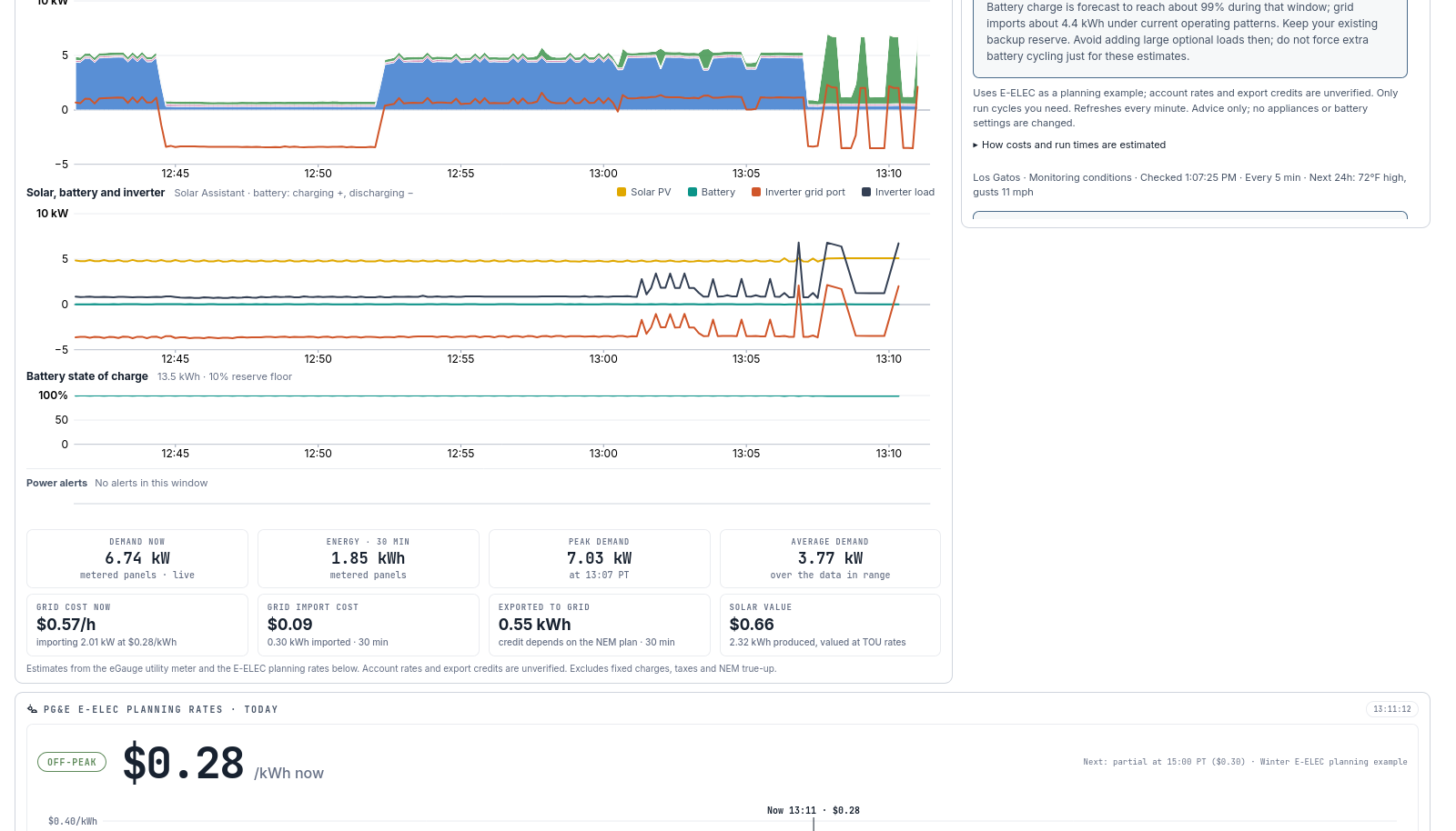
`03_general_detail_series.png`	Solar, battery and inverter series, state of charge and planning rates
`04_anomalies.png`	Anomalies tab: critical issues, relay log and event history
`05_appliances_nilm_heatmap.png`	Appliances tab: live NILM decisions per panel, written by the inference engine (Nemotron, with BiLSTM fallback)
`06_appliances_all_22_heads.png`	All 22 appliance heads across the three panels, idle ones included
`07_ask_nemotron.png`	Ask tab: grounded questions to the local Nemotron 3.5 Lightning, with preset operator questions
`08_predictions_power_outlook.png`	Predictions tab: per-channel 24-hour power forecasts with uncertainty bands
`09_predictions_battery_outlook.png`	Battery charge and temperature forecasts
`10_system_map.png`	System map: the verified deployment graph
`11_weather_readiness.png`	Weather tab: temperature and irradiance, history and forecast
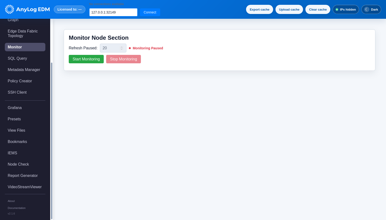
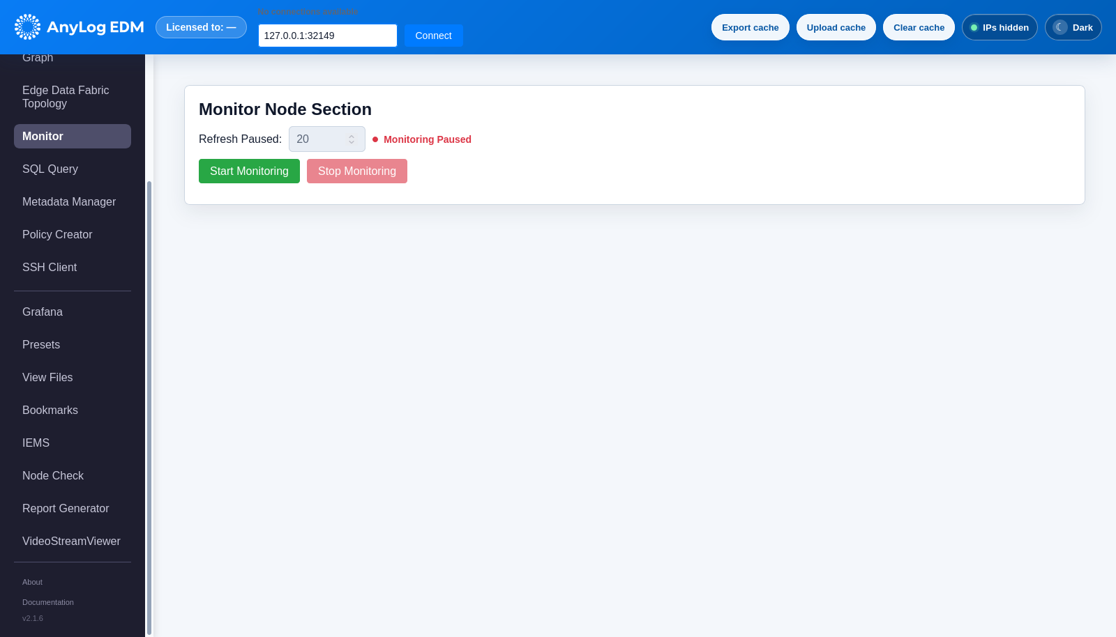
`12_anylog_remote_gui.png`	AnyLog remote GUI connected to the operator node (Monitor view)
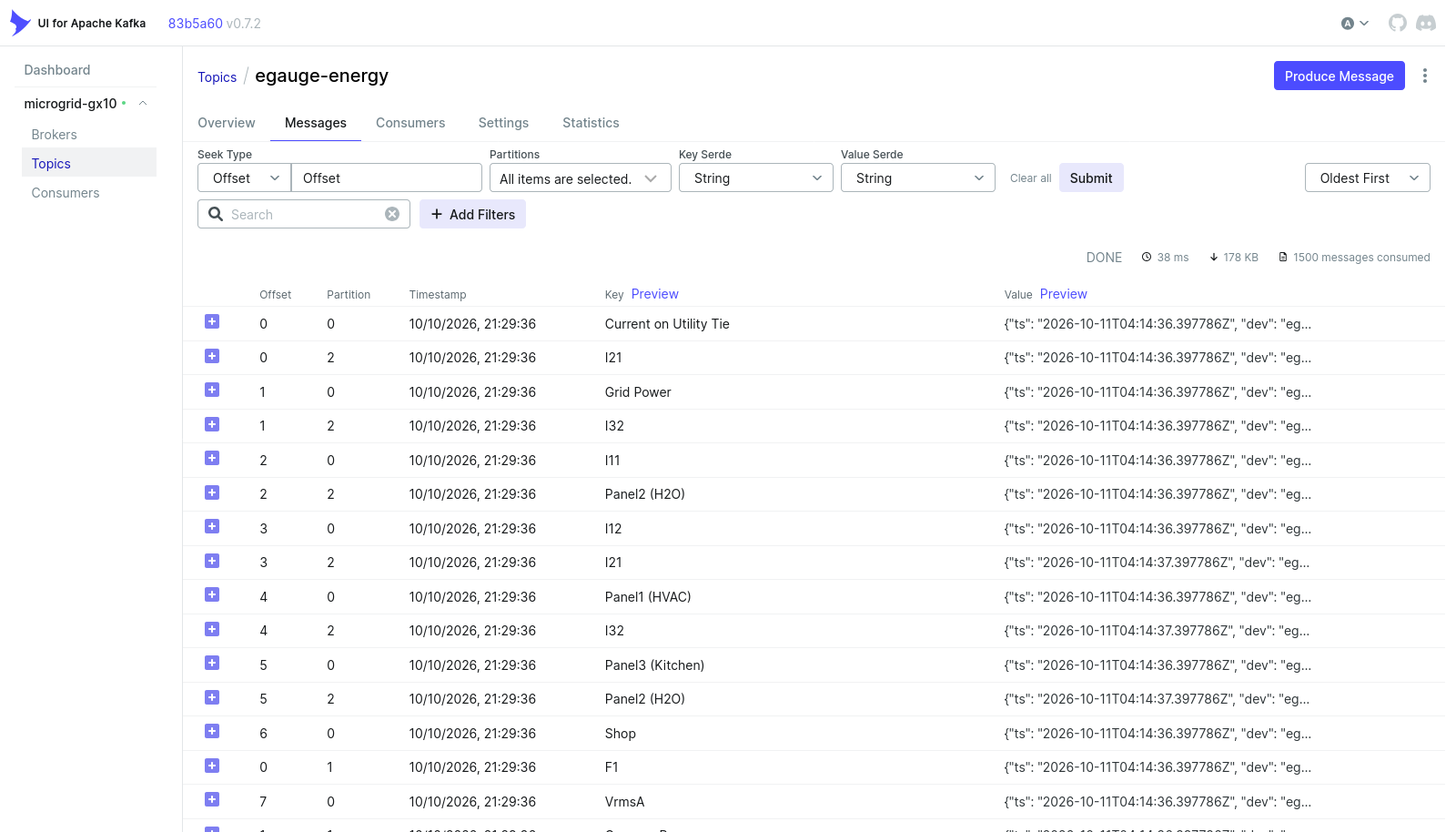
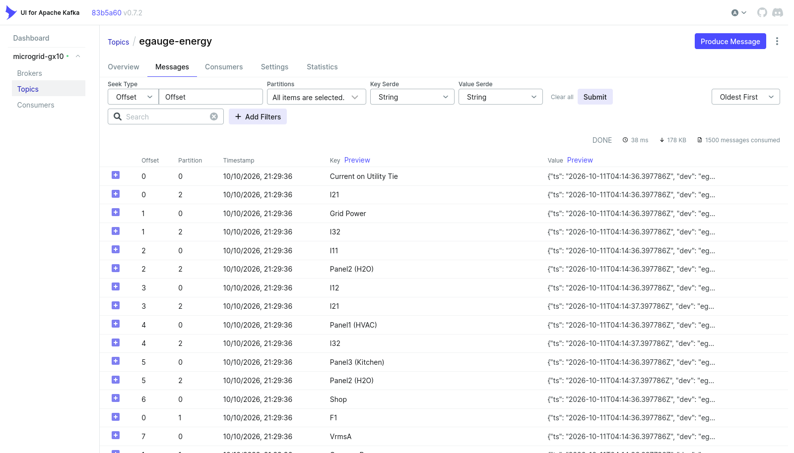
`13_kafka_ui.png`	Kafka UI: live messages on the `egauge-energy` topic
`14_appliance_forecaster.png`	Appliance-usage forecaster: 24-hour P(on) heatmap, model leaderboard and hot swaps