logo
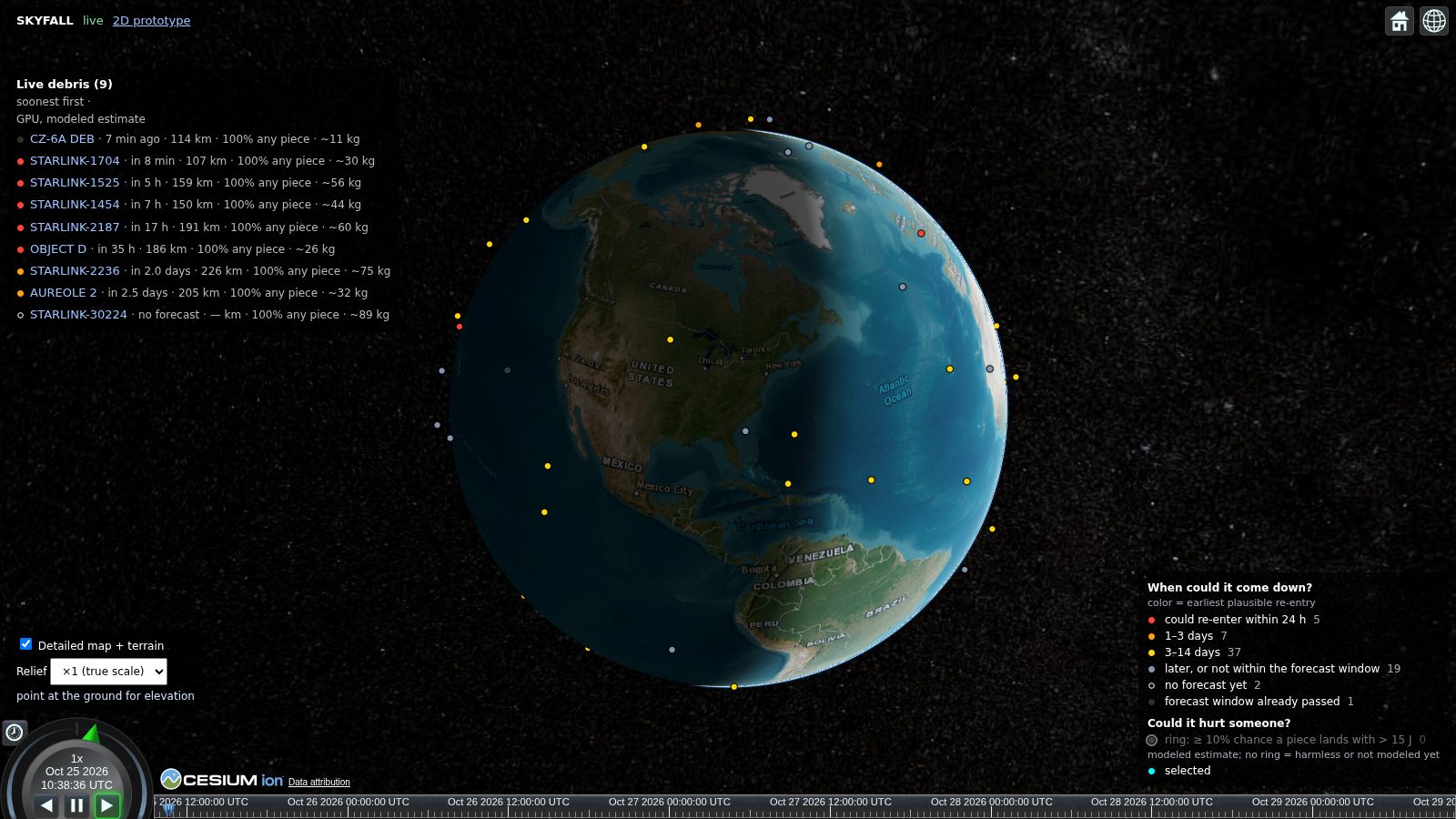
globe view
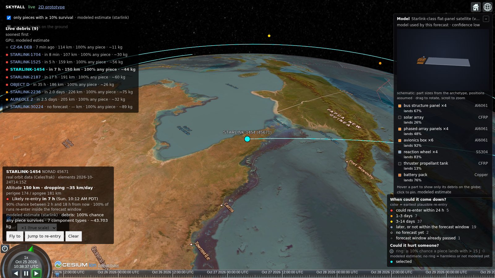
object breakdowns
impact zones
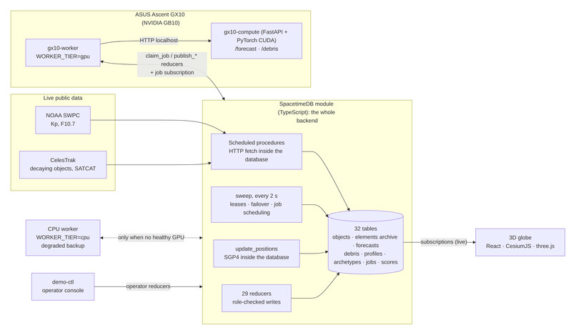
architecture

Inspiration

In March 2024, a piece of a discarded ISS battery pallet survived re-entry and crashed through the roof of a house in Naples, Florida. Thousands of objects are decaying out of orbit right now. Low Earth orbit holds thousands of short-lived satellites; Starlink alone de-orbits satellites almost daily, and rocket stages and old debris come down too. The public answer to "what's coming down, and where?" is usually a single date with a window of hours, and no idea what actually survives. Break-up and survivability analyses stay inside agencies.

We wanted to build the tool we wished existed: a live globe that shows which objects are re-entering, which pieces survive, how heavy and how dangerous they are, and where they could land, with honest uncertainty.

What it does

SKYFALL runs that analysis openly and continuously, on live public data:

Track every decaying satellite and rocket body from live orbit data (CelesTrak) and space weather (NOAA SWPC).
Forecast when and where each one re-enters, as a probability distribution from about 20,000 simulated futures per object.
Break it up into its components (bus, solar arrays, tanks, reaction wheels, batteries, engine parts) and fly every piece down through the atmosphere with heating and melting, thousands of times.
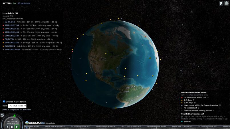
Show it all live on a 3D globe.

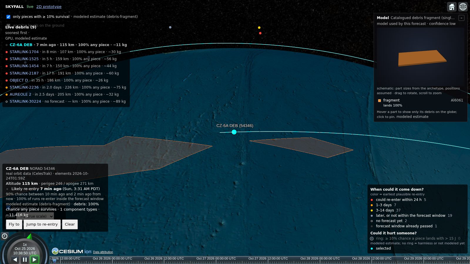
Each object is colored by its earliest plausible re-entry, so anything that could come down within a day stands out. A ring marks objects with at least a 10% chance that a piece lands with more than 15 J of energy, the usual threshold for a dangerous fragment. Clicking an object shows:

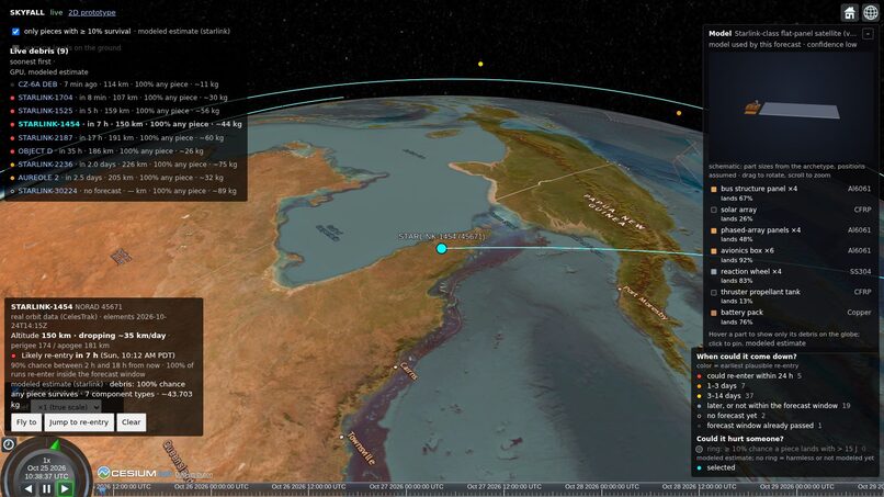
its live altitude, drop rate, and a probabilistic re-entry window, with a ground corridor that widens as uncertainty grows,
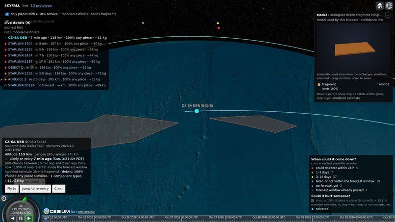
impact zones (50% and 90%) where surviving debris could fall, computed from thousands of simulated descents,
a 3D model of its components, each with its chance of reaching the ground, surviving mass and impact energy. Hover a part and the globe shows only that part's debris tracks and zones.

Forecasts update live as new orbit and space-weather data arrive. If our GPU goes down, the system fails over to CPU automatically and keeps forecasting. Every debris number is labeled as a modeled estimate.

How we built it

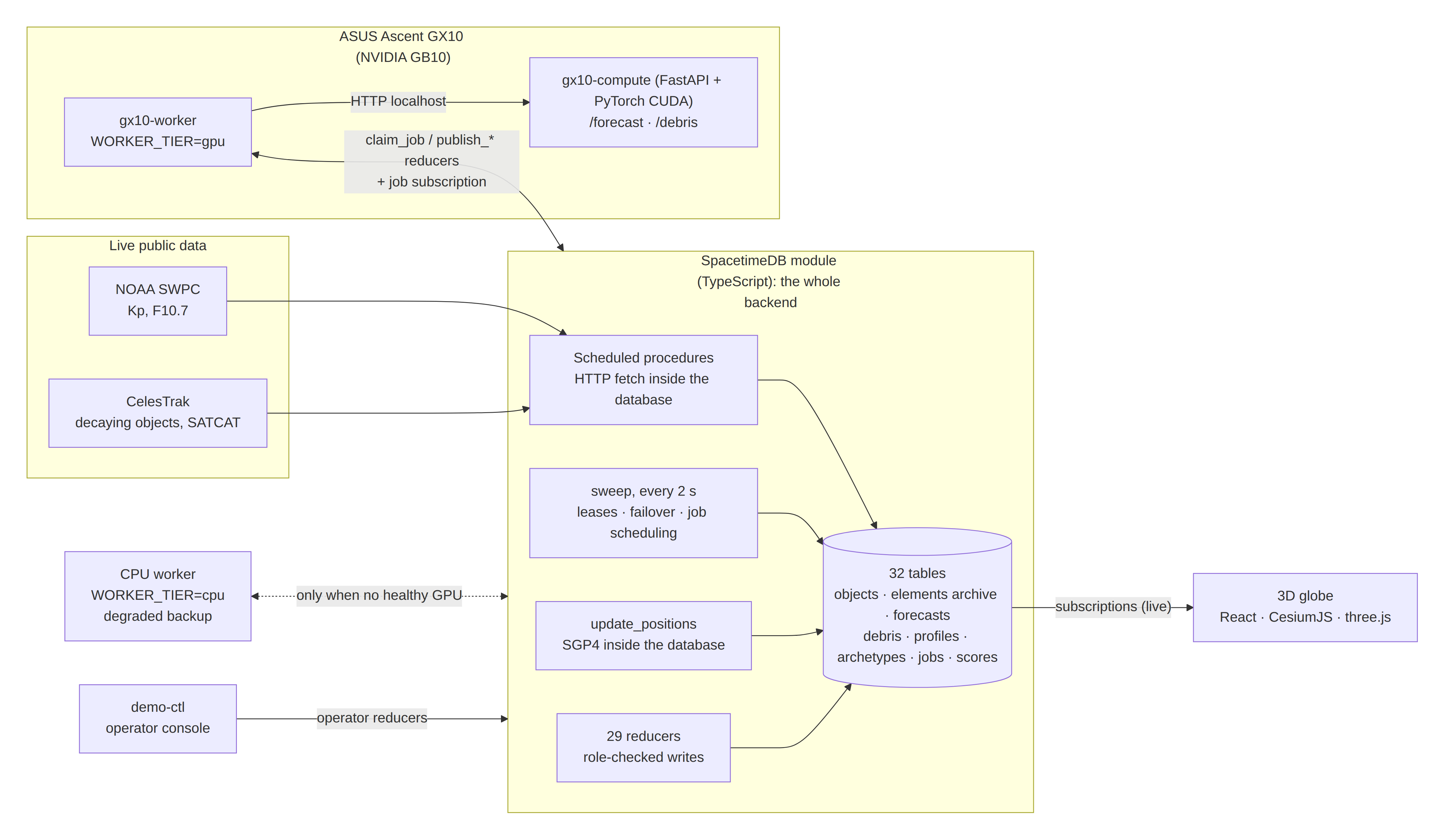
SpacetimeDB is the entire backend. It isn't just storage; it's the orchestrator. There is no other server, no side database and no message queue. One TypeScript module (about 2,400 lines: 32 tables, 29 reducers, 4 procedures, 6 schedules) does all of this:

Ingest: scheduled procedures make outbound HTTP calls from inside the database to poll NOAA SWPC space weather (every 15 min), CelesTrak decaying objects (every 2 h) and SATCAT decay dates (every 6 h).
Job queue with leases: forecast and debris jobs run in two lanes per worker (one bulk job, one fast job), with lease expiry, retries and oldest-first ordering. A scheduled sweep reducer requeues expired leases and evicts silent workers every 2 seconds.
Failover as a database rule: CPU workers get no jobs while a healthy GPU worker exists, so failover happens with no extra coordinator. Measured: after we killed the GPU worker, the CPU worker finished the next job 7 seconds later.
Chaining: publishing a forecast versions and archives it, then automatically queues a debris job when the chance of re-entry within 72 h is at least 20%.
Orbits in the database: SGP4 runs inside the module to keep every object's live position current.
Self-scoring: when an official decay date arrives, the module scores the last forecast made before it (hours of error, inside the window or not, lead time).
Streaming: the web client subscribes to the tables directly, so the globe updates the moment a result lands, with no polling and no API layer.

The workers are stateless. Kill one mid-job and the database requeues the job and someone else finishes it.

Forecast physics (GPU Monte Carlo on an ASUS Ascent GX10). Each object starts from its SGP4 state and is propagated with RK4 under Earth's oblateness ($J_2$) and atmospheric drag against a co-rotating atmosphere:

$$ \mathbf a_{\text{drag}} = -\frac{1}{2}\frac{C_D A}{m}\rho(h,t)\left|\mathbf v_{\text{rel}}\right|\mathbf v_{\text{rel}} $$

Density $\rho$ comes from the NRLMSIS 2.1 atmosphere model, driven by live solar (F10.7) and geomagnetic (Ap) indices. We don't trust a single ballistic coefficient. We calibrate drag per object so its simulated decay matches the decay actually observed in its orbital elements. Then we run about 20,000 particles per object, each with its own perturbed drag and position: the drag spread widens when Kp is high, and the position error grows with the age of the elements. All particles are batched in PyTorch on the GPU. The re-entry window is the spread of the particles:

$$ P(t_{\text{reentry}} \le t) \approx \frac{1}{N}\sum_{i=1}^{N} \mathbf{1}\left[t^{(i)}_{\text{reentry}} \le t\right] $$

Ground sightings can be fused by Bayesian updating with adaptive importance sampling, so corridors narrow as evidence arrives.

Debris survival model. Each object is split into a documented archetype's components. There are nine archetypes so far (Starlink-class, 3U/6U CubeSats, microsat, large satellite, cargo vehicle, rocket upper stage, and others), each with its material, shape, mass, size and sources. Starting from each particle's state at 80 km, every (particle × component) flies its own 3-DOF trajectory on the GPU with stagnation-point heating from the Sutton–Graves relation:

$$ \dot{q} = k\,\sqrt{\frac{\rho}{r_n}}\;v^{3} $$

A component demises if the absorbed heat exceeds what it needs to reach its melting point and melt:

$$ Q_{\text{demise}} = m\left[c_p\,(T_{\text{melt}} - T_0) + L_f\right] $$

The model covers seven materials (aluminium, titanium, stainless steel, CFRP, glass, copper, Inconel) and includes radiative cooling. Survivors are carried to the ground, where we record impact speed, energy and 50%/90% footprint zones. It's a reduced version of the object-oriented approach used by NASA DAS and ESA DRAMA.

What the GX10 made possible. From our live database so far:

32.7 million simulated futures and 752 billion particle integration steps
about 48 million particle-steps per second, roughly 22× faster than the CPU fallback
largest single run: 71 objects × 20,000 particles, 62.8 billion steps
196 full debris break-up runs

That's what lets us rerun tens of thousands of futures for every decaying object every 20 minutes, plus a full break-up for each object about to come down.

Frontend. A React + CesiumJS 3D globe subscribed live to SpacetimeDB:

city-level imagery and 3D terrain
re-entry coloring with a filterable legend and uncertainty corridors
debris tracks, footprints and ground warning levels
a three.js viewer that draws each object's archetype as an interactive 3D schematic

Tools. Cursor was our core AI coding agent. Its cloud agents opened branches directly against the repo, including our final-hours fixes and a benchmark of the forecast engine on the GX10.

Grok worked at two levels:

Grok Bot handled automation and project management. It ran a small team of agents: one for prize strategy and design, one for deployment and our domain, and one for SpacetimeDB. It also launched the Cursor cloud agents.
Grok 4.7 inside Cursor built our forecast-validation layer in SpacetimeDB: decay outcomes, the SATCAT fetch, forecast scoring and historical replay.

Challenges we ran into

Re-entry is hard to predict. Atmospheric density can swing a lot with solar activity, and small errors in drag compound over days. Against official re-entry predictions, our early forecasts ran 7 to 11 hours late. We'd rather show that honestly than hide it, and per-object drag calibration was our biggest fix.
Ground truth is scarce. Validating against past re-entries means using only the orbital data available before the event. Historical element sets and recovered-debris locations are hard to find, so building fair test cases was a project in itself.
Object physical data is incomplete. Mass, shape and materials aren't public for most objects, so we built sourced archetypes, label every number as real, modeled or assumed, and show a confidence rating.
Making failover trustworthy. Getting leases, heartbeats and requeues right, so no job is lost or run twice when the GPU drops, took several iterations.
Making debris physics fast enough to run continuously. Batching every particle × component × time step into GPU tensors turned a one-off analysis into something we run for every object about to come down.
Time. We built a database-driven job system, two GPU physics engines and a live 3D frontend in one weekend.

Accomplishments that we're proud of

A complete live pipeline, from public feeds to GPU physics to a 3D globe, with SpacetimeDB as the only stateful component.
GPU-to-CPU failover in 7 seconds, coordinated entirely by database rules.
Hundreds of billions of physics steps on a desk-side GX10.
Forecasts that score themselves against official decay dates.
A per-component survivability view of live re-entries, something the public hasn't had before.

What we learned

A real-time database can be the whole backend: ingestion, scheduling, job orchestration, failover, archiving and streaming, with no separate queue or worker coordinator. It made failure handling simpler, not harder.
How much re-entry prediction depends on the atmosphere, and why showing uncertainty matters more than a single confident answer.
How to write physics that runs fast in parallel on a GPU, and how to keep a CPU path that runs the same physics, visibly degraded, when the GPU is gone.
How to work with AI agents as teammates: Grok Bot for planning and coordination, and Cursor for writing and reviewing code.

What's next

Hindcast validation at scale: our forecasts are already scored against official decay dates in the database. Next is a public scorecard comparing us to official predictions over many past re-entries.
Better object data: Space-Track and DISCOSweb for real object mass, shape and materials, and more archetypes (Long March stages, Falcon 9 second stage, OneWeb, Kuiper, Starlink v2 mini).
Better atmosphere: density that varies with latitude and local time, time-varying solar activity, a spread of break-up altitudes, and winds for light debris.
Population-weighted casualty risk under each footprint.