-
-
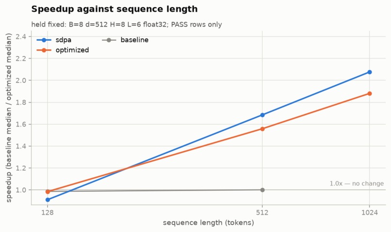
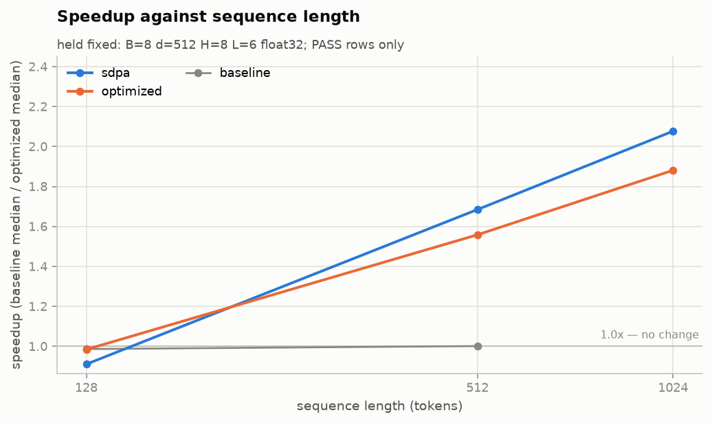
Attention's share of the work grows with sequence length: the fused kernel loses at S=128 (0.910×) and reaches 2.077× at S=1024.
-
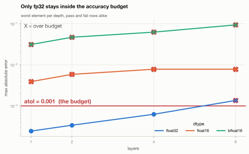
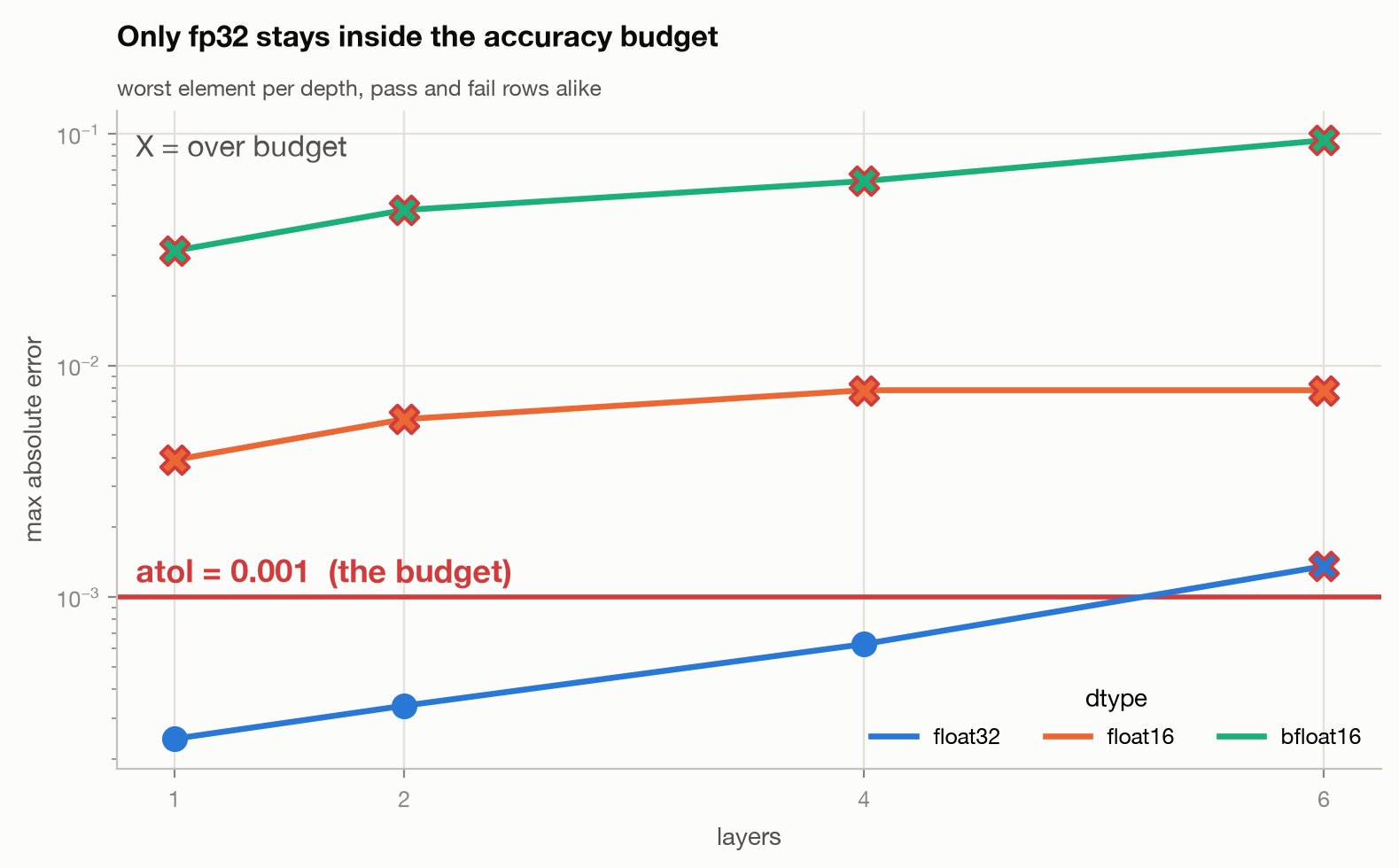
fp16 and bf16 exceed the 0.001 absolute budget at every depth. fp32 crosses only at six layers, where the relative rule carries it.
-
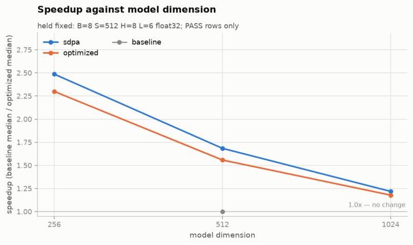
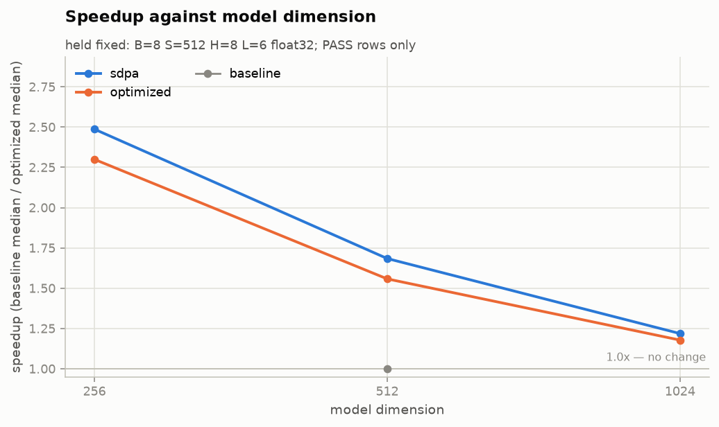
Widening the model shrinks attention's share, since projections grow as d² — so the gain falls from 2.487× at d=256 to 1.219× at d=1024.
-
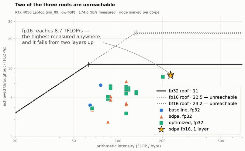
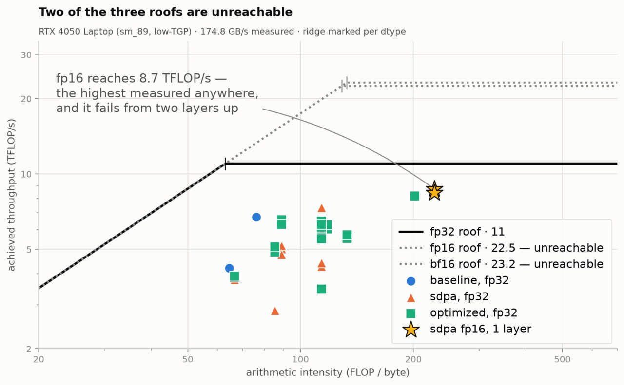
Measured peaks put the fp32 ridge at 62.9 FLOP/byte. The fp16 and bf16 roofs are real but unreachable — neither passes the tolerance.
-
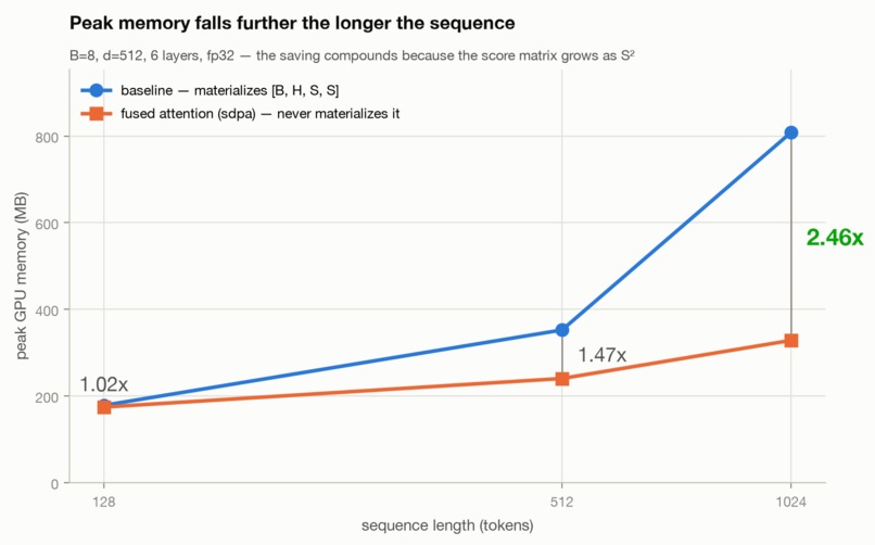
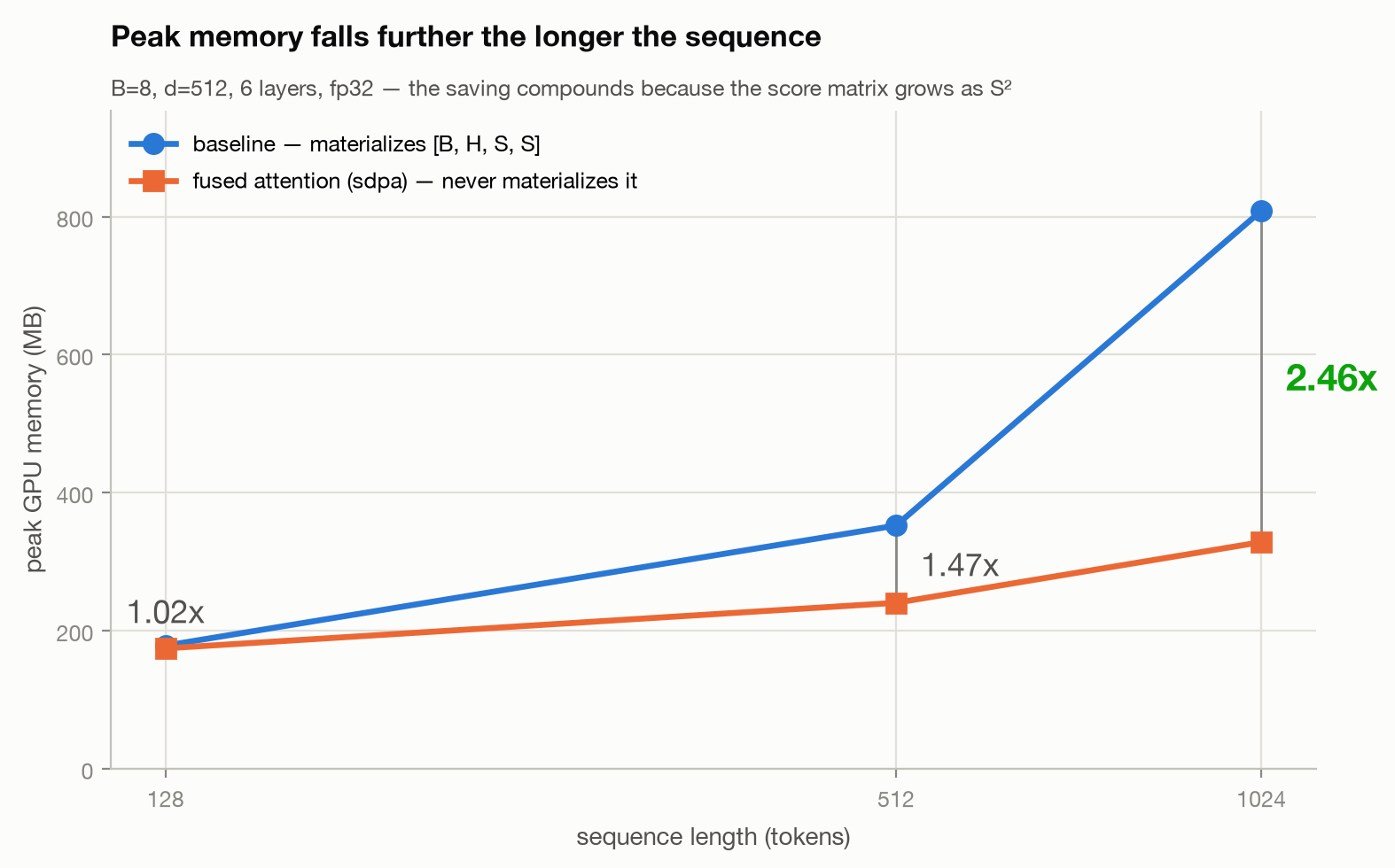
The score matrix grows as S², so the saving compounds: the fused path uses 1.02× less memory at S=128 and 2.46× less at S=1024.
Inspiration
The challenge gave us a working Transformer and asked us to replace exactly one method, as long as the output still matched the reference element by element. That constraint is what drew us in. Our job was not to write a fast kernel, it was to write one that was provably still computing the same thing.
The first question we asked was why attention is expensive at all, and we found the quadratic cost is not intrinsic to the operation:
$$\text{Attention}(Q,K,V) = \text{softmax}!\left(\frac{QK^{\top}}{\sqrt{d_k}}\right)V$$
Strip the softmax and this is a product of three matrices, and matrix multiplication is associative — \( (QK^{\top})V \) costs \( O(S^2 d) \), but \( Q(K^{\top}V) \) costs only \( O(S d^2) \). We realised the softmax is the only reason the cheaper grouping is illegal. It sits between the two products as a nonlinearity, so the \( S \times S \) score matrix has to exist.
Reading the reference implementation, we saw it building that matrix explicitly and computing the softmax over it in fp32 even when the model ran in half precision. That one design choice told us where the time was likely going, and it set the direction for everything we did afterwards.
What it does
We replaced the Transformer's forward pass with a fused attention kernel, and this is the part that mattered most. We made the model decide per input shape whether to use it at all.
We found the fused kernel was not universally better. We measured the same kernel at 0.910× at \(S=128\), genuinely slower than the reference, and at 2.077× at \(S=1024\). Attention is a small fraction of the work on a short sequence and most of it on a long one, so we concluded a single implementation would be the wrong answer at one end or the other.
Our shipped model reads the incoming tensor and routes accordingly. We ordered the rules so correctness gates come first and performance rules second:
| # | Condition | We route to | Why |
|---|---|---|---|
| 1 | No CUDA device | reference | we could not test that path |
| 2 | bfloat16 |
reference | fails tolerance at every depth |
| 3 | float16, \(L \ge 2\) |
reference | fails tolerance from two layers |
| 4 | causal, \(L \ge 6\) | reference | passed only 21 of 40 seeds |
| 5 | batch \(= 1\) | reference | we measured 0.853× — a regression |
| 6 | \(S \le 128\) | reference | we measured 0.910× — a regression |
| 7 | otherwise | fused kernel | we measured it faster |
Routing changed the aggregate in a way we think is the right trade. On its own the fused kernel reached a geometric mean of 1.531× but bottomed out at 0.853× on the shapes where it lost. Our routed model gave up some of that peak — 1.322× geometric mean, 2.300× best case — and in return never dropped below 0.984×. We turned a kernel that sometimes made things worse into a model that essentially never does.
Every configuration we report passes the stricter of the two published tolerances, \( \text{atol}=0.001 \) and \( \text{rtol}=0.01 \), rather than the looser \( 0.002 / 0.02 \) from the problem statement.
How we built it
We profiled before we optimised anything. We measured the baseline at three shapes and let that profile decide the order of the work. At the shapes where speedup mattered, kernel launches accounted for 3.45% and 0.80% of wall time, so we ruled out launch overhead as the constraint and put fusion ahead of any attempt at CUDA graphs.
We worked out the ceiling before we measured the result. Counting FLOPs per layer:
$$\underbrace{8BSd^2}{\text{Q, K, V, output}} \;+\; \underbrace{4BS^2d}{QK^{\top},\; PV} \;+\; \underbrace{4BSdf}_{\text{FFN}}$$
At \( B=8,\ S=512,\ d=512 \) we calculated attention as 14.3% of the forward pass. By Amdahl's law, that meant making it infinitely fast could give us at most:
$$\frac{1}{1 - 0.143} = 1.167\times$$
Then we measured 1.684×. We could not explain a speedup above that ceiling by removing arithmetic, because there was not enough arithmetic there to remove. Inverting Amdahl told us attention must have occupied 40% of the runtime — 2.8× its share of the FLOPs. We took that as direct evidence the real cost was memory traffic: writing and re-reading the \( [B, H, S, S] \) score matrix rather than doing the two matrix products.
Our roofline analysis reached the same conclusion by a different route. We microbenchmarked the card rather than trusting the datasheet — 11.0 TFLOP/s fp32 with TF32, 174.8 GB/s bandwidth — which put the ridge point at 62.9 FLOP/byte. We then found the reference's arithmetic intensity falls as sequences grow, because the score matrix grows faster than the useful work:
| \(S\) | Reference | Fused |
|---|---|---|
| 128 | 76.2 | 88.9 |
| 512 | 64.6 | 113.8 |
| 1024 | 52.0 | 133.2 |
| 2048 | 40.5 | 168.6 |
The reference crosses below the ridge into the bandwidth-bound region between \(S=512\) and \(S=1024\), while our fused path moves the opposite way. An analytic byte count and a stopwatch had independently told us the same thing.
We treated the measurement apparatus as part of what we were building. We kept results in an append-only log where every row records the commit it came from, and made the harness refuse to run against uncommitted changes. We added a memory pre-check that predicts VRAM before a configuration runs, so an impossible shape gets recorded as skipped instead of killing an unattended sweep. We logged GPU clocks during every run and threw out any run whose clock fell below 85% of its opening value, because we were measuring on a laptop GPU that throttles. We ran our 286-test correctness suite on a second machine with no GPU at all.
Challenges we ran into
Our first baseline was wrong. Our initial profiling run reported 18.6 / 64.6 / 215.2 ms. We had never set matmul_precision="high" or allow_tf32=True in the standalone profiler, both of which the organizers' script enables by default, so we were running fp32 matmuls at 5.7 TFLOP/s while our benchmark harness ran the same code at 11.0. Once we matched the global state we got 13.5 / 52.1 / 176.5 ms, and the runtime-API kernel count per forward dropped from 115 to 67. We expected identical kernels to simply run faster, since TF32 is a math mode rather than a storage format. Instead PyTorch selected entirely different tensor-core kernels. A flag we had read as a precision setting turned out to be a kernel-selection setting.
We could not ship reduced precision, and the reason was not a bug in our kernel. bf16 failed at every depth we tried. We traced the worst element to exactly 2 ULP of bf16: the format stores 7 mantissa bits, so at magnitude 2.17 one ULP is \( 2^{1-7} = 0.015625 \), and we measured an error of 0.03125 — 1.44% relative against a 1% tolerance.
We found the cause in the reference itself. It rounds the softmax probabilities to the model dtype before the \( PV \) product, while our fused kernel keeps them in fp32 throughout. Our path is more accurate; it simply does not reproduce the reference's intermediate rounding. Working it back, a 1% relative tolerance at that magnitude is 1.389 ULP of bf16 — tighter than the format's own granularity. We concluded that only an implementation reproducing the reference's exact operation order could pass, which is precisely what an optimised kernel must not do.
fp16 gave us more room, with 10 mantissa bits putting the same 2 ULP at 0.18%. It passed at one layer at 2.020× and failed from two, once error had compounded through the residual stream. At the benchmark's default depth of six layers we were left with fp32 as the only shippable dtype, which meant giving up the roughly 2× throughput the hardware offers in half precision.
We lost per-kernel attribution to a platform limitation. Under WSL2, CUPTI does not populate device-side kernel completion records, so our exported traces contained the full CPU-side story and no kernel entries at all. We had to make our analysis distinguish "unmeasurable" from "zero", since a 0% GPU-busy reading would have looked like a catastrophic result rather than a missing one. We substituted launch-count arithmetic from the CPU-side track. Our latency numbers were unaffected, because cuda.Event timing lives on the CUDA stream and does not depend on the profiler backend.
Some of our results turned out to be seed luck. One causal configuration first measured 2.124× and 1.778×. When we re-ran it across 40 seeds it passed only 21 of them. We kept those rows in the log, superseded by their corrections, and now route that configuration to the reference.
Accomplishments that we're proud of
We beat the ceiling our own arithmetic allowed. Predicting 1.167× from FLOP share and then measuring 1.684× did not mean we had written a better kernel — it told us our model of where the time went had been wrong in a way we could identify and name. We had recorded the prediction before taking the measurement, and our roofline reached the same conclusion independently.
We used dispatch to remove regressions rather than to chase peaks. Our geometric mean falling from 1.531× to 1.322× looks like a loss until the worst case is read alongside it, moving from 0.853× to 0.984×. Across a benchmark spanning many shapes, we decided never being slower was worth more than occasionally being faster.
We stated a negative result precisely enough to be useful. "bf16 does not work" would have been an anecdote. "The worst element is 2 ULP, the tolerance is 1.389 ULP, and therefore no reordered computation in this format can pass" is a property of the benchmark that anyone can check for themselves.
We made every number reproducible from a clean clone. We kept the organizers' file byte-identical to the download, pinned its SHA-256, and enforced that with a test. Every figure, table and number in our report comes out of one command run against the append-only log. Our control strategy — an unmodified copy of the reference — measures 0.994×, which is how we know the measuring rig itself is honest.
What we learned
Profile first, and believe the profile. We had assumed small shapes would be dominated by kernel launch overhead. The measurement disagreed, and following our assumption instead would have cost us a day on CUDA graphs that bought very little.
The ridge point moves with precision, and it moves right. We found reduced precision raises the compute roof and does nothing at all for the bandwidth roof, pushing the crossover from 62.9 to 132.7 FLOP/byte. That means switching to a smaller dtype can make a workload more memory-bound rather than less. A kernel does not simply move up the roofline chart — it can cross to the other side of the ridge, and the right next optimisation changes with it.
A tolerance can be tighter than a format's own precision. We had expected our accuracy limits to come from our implementation. In half precision they came from the interaction between the tolerance and the number format, and no correct implementation could have satisfied them.
Correctness did not fit the abstraction we had built for performance. We keyed our dispatcher on tensor shape, reasoning that depth changes how long a forward pass takes but not which kernel suits a shape. That held for performance and failed for correctness, because fp16 is admissible at one layer and not at six. We had to move the depth rule into the entry point that knows the model configuration, rather than the shape-based router.
A baseline is a measurement too. Ours was wrong for a while, and we only caught it because two of our tools disagreed — neither looked suspicious on its own.
What's next for Shape-Aware Attention
Fusing LayerNorm. With reduced precision closed off to us, this is one of the few remaining sources of gain. Now that the score matrix no longer crosses memory, what is left is the FFN products and the elementwise traffic between them — we are reaching 5.0–6.4 TFLOP/s against an 11.0 TFLOP/s roof, so roughly half of achievable peak is still on the table.
Pushing to longer sequences. Our memory model says the reference needs about 9.1 GiB at \( S=8192 \) against a 6 GB card and cannot run at any batch size, while our fused path never materialises \( [B, H, S, S] \) at all. That would give us a categorical result rather than a ratio: not "ours is faster" but "ours runs where the reference cannot."
CUDA graphs for the small-shape case. We measured launch overhead at 13.75% of wall time at the smallest shape, which left the question undecided rather than settled — and that is the one regime where our fused kernel still loses.
Measuring the other architectures. We correctness-tested the sm_75 and sm_80 paths by forced dispatch, but we never performance-measured them because we had one GPU between us. We do not claim they are faster there, and closing that gap needs hardware rather than code.


Log in or sign up for Devpost to join the conversation.