Green ML

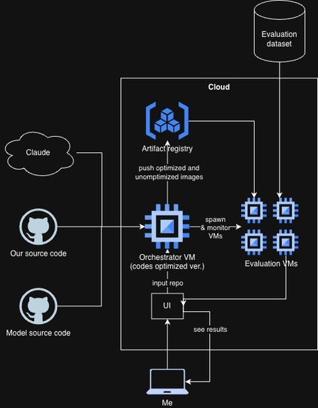
Flowchart

GreenML - Trimming the model, trimming the emissions

Inspiration

We chose to treat sustainability not as a hardware limitation, but as software engineering debt. In the era of massive AI, "clean code" must evolve beyond readability to mean carbon-efficient execution.

While the hardware and the power grid are static environments, the software is the dynamic variable we can actually control. We were inspired to treat every redundant flop or inefficient gradient transfer as a critical bug—a literal leak of planetary resources that software has the power to patch across an entire cluster with a single deployment.

The question that inspired this project was simple:

"If we optimize an ML model for speed, how much carbon do we actually save — and does the answer change depending on which GPU or which country you run it in?"

The answer, it turns out, is not straightforward. It requires bridging three worlds: software engineering, cloud infrastructure, and environmental science. That's what this pipeline does.

What We Built

We built an end-to-end automated pipeline that takes any ML model repository as input and produces two things: a faster, optimized version of that model, and a rigorous carbon comparison between the two.

The key output is two SCI scores — one measured on the original, unoptimized model, and one measured after the pipeline has applied its improvements. The difference between them is the carbon cost of the inefficiency: concrete, quantified, and expressed in gCO₂ per inference rather than in abstract compute metrics.

The pipeline has seven stages:

Download — Clone a target ML repo given a paper or GitHub link.
Containerize (baseline) — Build an unoptimized Docker container from the repo as-is.
Inspect & Plan — Use the Claude API to read the codebase and identify performance optimizations (quantization, mixed precision, batching, kernel tuning) that preserve accuracy.
Optimize — Apply the changes automatically, with a written explanation of what changed, why, and what the expected impact is. If the build breaks, the Claude API self-heals it. All changes, decisions, and self-healing actions can be used to understand what the model was doing wrong, how it was fixed, and what to carry forward into future work.
Containerize (optimized) — Build the optimized Docker container.
Benchmark — Deploy both containers to multiple GPU instances on a cloud provider (A100, H100, B200), measuring CPU, GPU, RAM utilization, wall time, and accuracy against the original paper's dataset. The SCI score is computed for both the unoptimized and optimized containers at this stage.
Report — Compile a full comparison: accuracy, performance, and the delta in planetary impact between the two versions — expressed as $\Delta\text{SCI} = \text{SCI}{\text{before}} - \text{SCI}{\text{after}}$.

Translating Compute to Carbon: The SCI Score

The core scientific contribution of the pipeline is translating raw compute metrics into carbon impact using the Green Software Foundation's SCI specification.

For each benchmarked run, we compute:

$$O = E \times I$$

$$M = TE \times \frac{T_{iR}}{L \times 8760}$$

$$\text{TotalCarbon} = O + M$$

$$\text{SCI} = \frac{\text{TotalCarbon}}{R}$$

Where:

Symbol	Meaning	Source
$E$	Energy consumed (kWh)	CodeCarbon
$I$	Carbon intensity (gCO₂eq/kWh)	Electricity Maps API
$T_{iR}$	Runtime (hours)	CodeCarbon
$R$	Functional units (e.g. inferences)	Workload output
$TE$	Total embodied carbon of the GPU (gCO₂eq)	Manufacturer LCAs
$L$	GPU lifespan (years)	Hardware specs

The operational carbon $O$ captures the electricity cost of the run, adjusted for the real-time carbon intensity of the grid where the workload ran. The embodied carbon $M$ allocates a fair share of the GPU's manufacturing footprint to this specific run, proportional to the fraction of its lifetime hours consumed.

This gives us two SCI scores per experiment — one before optimization, one after — making the carbon savings of the optimization directly quantifiable:

$$\Delta \text{SCI} = \text{SCI}{\text{before}} - \text{SCI}{\text{after}}$$

The Location Dimension

One of the most surprising insights was how much grid location dominates the operational carbon. The same model, running the same workload on the same GPU, can have a 100× difference in $O$ depending on whether it runs in France (low-carbon nuclear grid) versus Poland (high-carbon coal grid).

This led to a third SCI score in our pipeline: after the software optimization, we use a location optimization tool to identify the lowest-carbon grid zone available, producing an even further reduced SCI — purely from moving the workload geographically, with no code changes at all.

How We Built It

The pipeline is fully modular:

pipeline/
├── modules/
│   ├── downloader.py       # Repo cloning
│   ├── docker_builder.py   # Container builds + self-healing via Claude API
│   ├── optimizer.py        # Optimization planning + code changes via Claude API
│   ├── benchmarker.py      # Cloud GPU deployment + metric collection
│   ├── carbon_metrics.py   # SCI computation (CodeCarbon + Electricity Maps)
│   └── reporter.py         # Final report generation

Carbon tracking is fully automatic — track_and_compute() wraps any workload callable, starts CodeCarbon, runs the workload, stops the tracker, fetches live carbon intensity from Electricity Maps, and returns the complete SCI breakdown in one call.

Challenges, Learnings & The Path to Scale

Building this pipeline taught us that the hardest problems were not the ones we expected.

Embodied carbon data is sparse. NVIDIA does not publish standalone GPU Life Cycle Assessment data. The $TE$ values for H100 and B200 in our pipeline are estimates extrapolated from partial server LCAs and academic literature (Gupta et al., HPCA 2022). This is an industry-wide transparency gap that needs to close before tools like ours can be fully rigorous.

CodeCarbon's default intensity is a global average. Without plugging in real grid data from Electricity Maps, the operational carbon estimate can be off by 100× depending on location. This is precisely the gap our $I$ integration addresses — and it highlights how easy it is to produce carbon numbers that look credible but are quietly wrong.

Determinism vs. flexibility in automated builds. The build stage must never fail silently. We handle this with a self-healing loop: if a container build fails, the Claude API reads the error, patches the code, and retries — ensuring the pipeline always produces a valid, comparable baseline.

Scale is where this product becomes meaningful. The core argument for scaling is simple: the tool's impact grows faster than its cost. One optimized model saves a little carbon. A hundred optimized models, running continuously across an organization's full AI portfolio, saves carbon at a rate no individual engineer or team could achieve manually. Scale is not just a feature — it is the point.

Step 1 — Harden the optimization quality Before scaling, the agent needs a reliable accuracy regression gate. If an optimization drops model accuracy beyond a defined threshold, it is automatically rejected and flagged. No human should need to catch this at scale. Step 2 — Integrate into CI/CD Connect the pipeline as a GitHub Action or GitLab CI step. Every pull request that touches model code triggers an automatic carbon benchmark. The SCI delta appears on the PR the same way test coverage does — making carbon a first-class metric in the development workflow. Step 3 — Build a central SCI registry Every run writes its SCI score to a central database, keyed by model, version, and hardware. This creates a time series of carbon efficiency per model — you can see whether each model is improving or regressing across releases, and where the biggest inefficiencies are hiding. Step 4 — Introduce tiered benchmarking Full GPU benchmarks are expensive. At scale, run fast proxy benchmarks first to filter bad optimizations early, and reserve full A100/H100 runs for candidates that pass. This is the same logic as CI/CD: cheap tests first, costly tests only when warranted. Step 5 — Add location-aware scheduling Combine SCI scores with live Electricity Maps data to route workloads to the lowest-carbon available region at any given hour. This reduces operational carbon with zero code changes — pure infrastructure intelligence. Step 6 — Track the pipeline's own carbon cost The pipeline consumes energy to run. Measure its own SCI so you can demonstrate that the carbon saved by optimizations always exceeds the carbon spent running the tool. This payback ratio is the key number that justifies the investment at scale. Step 7 — Report for compliance and stakeholders The SCI registry becomes an audit trail: every model, every version, every carbon score, timestamped and stored. As sustainability reporting requirements tighten (EU AI Act, CSRD), organizations running this pipeline already have the data they need — without any additional instrumentation.

The reason to scale this is not just efficiency. It is that the problems this tool solves — invisible carbon costs, unoptimized models, misallocated compute — are proportional to the size of an organization's AI footprint. The bigger the portfolio, the bigger the waste, and therefore the bigger the impact of fixing it systematically. A tool that saves 0.000008 gCO₂ per inference sounds small. Applied across billions of daily inferences across hundreds of production models, it becomes a meaningful, measurable contribution — the kind that shows up in an organization's emissions report, not just a hackathon slide.

What's next for Green ML

To maximize the impact of Green ML, we are shifting our optimization focus from individual units to massive GPU clusters, where even a 1% efficiency tweak in data synchronization scales into megawatts of power saved. By targeting the "idle energy" wasted during collective communication (All-Reduce) across thousands of nodes, we can slash the carbon footprint of LLM training at its most resource-intensive scale.