-
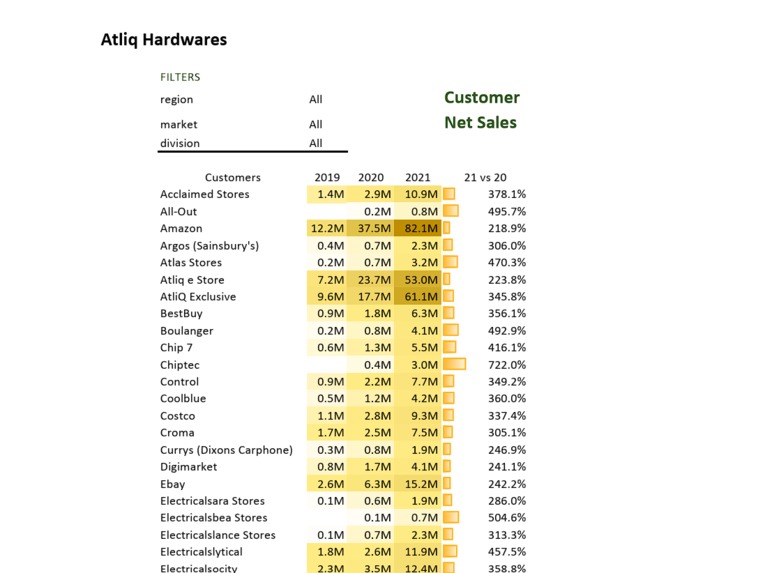
sales report
-
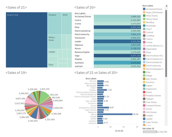
visualization using TableAu
InspirationCleaning Data Using Power Query:
a. Import your data into Excel.
b. Select any cell within your data range.
c. Go to the "Data" tab in the Excel ribbon and click on "From Table/Range" in the "Get & Transform Data" group. This will open Power Query Editor.
d. In Power Query Editor, you can perform various cleaning and transformation tasks.
e. Once you've finished cleaning and transforming your data, click on "Close & Load" to load the data back into Excel.
Creating a Report:
a. With your cleaned data loaded into Excel, you can now create a report.
b. Select any cell within your data range.
c. Go to the "Insert" tab in the Excel ribbon and choose the type of chart you want to create (e.g., a bar chart, line chart, or pie chart).
d. Excel will create a chart based on your data. You can customize the chart by modifying its title, axis labels, and other properties.
e. You can also create pivot tables to summarize your data further. Go to the "Insert" tab and select "PivotTable". Choose the data range and where you want the PivotTable to be placed, then click "OK". In the PivotTable Fields pane, drag fields into the Rows and Values areas to create your report.
f. Once you've created your report, you can further customize it by applying different styles, colors, and formatting options.
g. Finally, you can save your Excel file with the cleaned data and the report for future reference or sharing with others.
