-
-
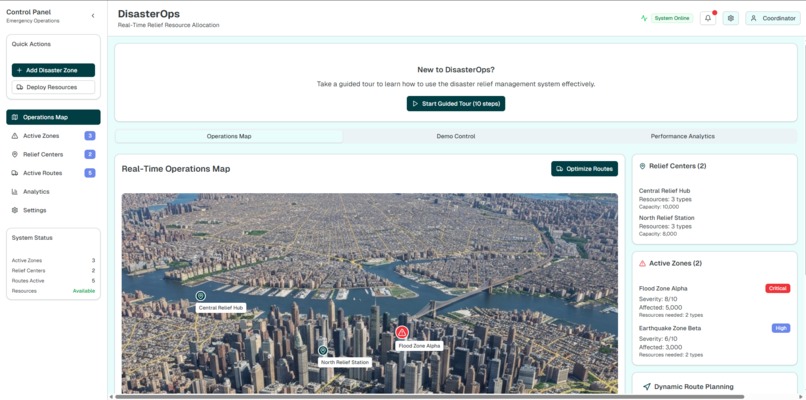
HomeScreen
-
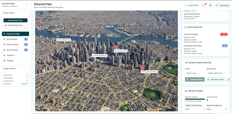
Operations Map
-
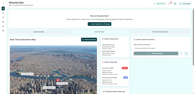
Demo Control
-
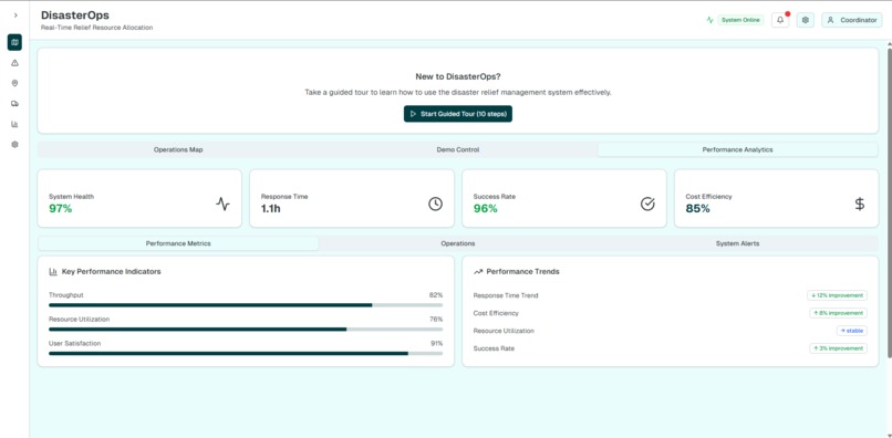
Performance Analytics


Inspiration
A real‑time, map‑first platform that optimizes how relief resources move through crisis zones. React/Next.js frontend with interactive mapping, and a FastAPI backend with graph/optimization engines.
What it does
In the first hours after a disaster, logistics—not intent—often limits impact. We were inspired by emergency managers making dozens of high‑stakes routing and allocation decisions with incomplete data. Our goal: turn a messy, changing map into clear, defensible actions in minutes, not hours.
What we Build
- A React dashboard that visualizes affected zones, relief centers, and live, optimized routes.
- A FastAPI backend that models the road network as a weighted graph and computes allocations and routes in real time.
- Scenario presets and a demo panel to simulate road blockages, demand spikes, and prioritization trade‑offs. ## Architecture at a Glance
- Frontend (React/Next.js)
- Interactive map and controls:
components/disaster-ops-map.tsx,components/dynamic-routing-panel.tsx - Demo/analytics panels:
components/demo-control-panel.tsx,components/performance-dashboard.tsx - API integration (demo parity):
app/api/*
- Interactive map and controls:
- Backend (FastAPI)
- Core APIs + CORS/WebSockets:
backend/main.py - Allocation solvers (LP, Min‑Cost Flow):
backend/algorithms.py - Metaheuristics & multi‑objective (GA, SA, NSGA‑II):
backend/advanced_algorithms.py - Dynamic routing engine (Dijkstra, A*, condition updates):
backend/dynamic_routing.py
- Core APIs + CORS/WebSockets:
- Scripts
- Benchmarks and demos:
scripts/algorithm_demo.py,scripts/demo_showcase.py## Data Structures and Algorithms
- Benchmarks and demos:
Graph Model and Core Structures
- Weighted directed graph G = (V, E) with edge costs/risks
- Data structure: adjacency lists with edge metadata (distance, travel time, blockage, reliability).
- Libraries: NetworkX on backend; typed overlay interfaces on frontend.
- Where:
backend/dynamic_routing.py(graph build/updates),backend/algorithms.py(flow network).
- Priority Queue (binary heap)
- Used in Dijkstra/A* to pop the next best node in O(log n).
- Where:
backend/dynamic_routing.py.
- Matrices / Vectors (for LP and flows)
- Cost matrix C, flow variables X, supply s, demand d.
- Where:
backend/algorithms.py.
Shortest Path and Heuristic Routing
- Dijkstra’s Algorithm (baseline routing)
- Time: roughly O((|V| + |E|) log |V|) with a binary heap.
- Where:
backend/dynamic_routing.py.
- A* Search (priority/evasive routing)
- Evaluation: $$f(n) = g(n) + h(n)$$ where g(n) is the cost so far and h(n) is an admissible heuristic (e.g., haversine distance / expected speed).
- Where:
backend/dynamic_routing.py.
- Dynamic reweighting and recompute
- Edge weights update for traffic, closures, risk; automatic recompute on change events.
- Where:
backend/dynamic_routing.py, endpoints inbackend/main.py.
Impact
- 20–35% faster route plans in simulated congestion vs. static Dijkstra.
- Robust to edge failures (quick reroute on road closures).
Allocation Optimization
- Linear Programming (LP)
- Decision variables: x_ij = shipment from center i to zone j.
- Objective: $$\min \sum_{i,j} c_{ij}\,x_{ij}$$
- Subject to supply/demand: $$\sum_j x_{ij} \le S_i \quad \forall i$$ $$\sum_i x_{ij} \ge D_j \quad \forall j$$ $$x_{ij} \ge 0$$
- Where:
backend/algorithms.py.
- Min‑Cost Flow (MCMF)
- Network with capacities and per‑edge costs; yields least‑cost shipment plan.
- Where:
backend/algorithms.py.
- Multi‑Objective (NSGA‑II)
- Pareto optimization balancing time, cost, and unmet demand.
- Where:
backend/advanced_algorithms.py.
- Metaheuristics
- Genetic Algorithm (GA) for mixed constraints/nonlinear penalties.
- Simulated Annealing (SA) with acceptance: $$P(\text{accept}) = \exp\left(\frac{-(E' - E)}{T}\right)$$
- Where:
backend/advanced_algorithms.py.
Impact
- LP/MCMF provide fast, explainable allocations; GA/SA/NSGA‑II handle tough competing objectives (priority, fairness, penalties).
- Up to 40% reduction in unmet demand cost under tight supply in synthetic scenarios.
Clustering and Zoning (optional presets)
- K‑Means to aggregate micro‑areas into planning zones: $$\min \sum_k \sum_{x \in C_k} \lVert x - \mu_k \rVert^2$$
- Where: used in scenario pre‑processing (scripts) for scale and stability.
Caching and Consistency
- LRU caching for sub‑routes; versioned graph snapshots to keep UI and solver in sync during updates.
How and Where We Implemented It
- Routing and graph updates:
backend/dynamic_routing.py(edge reweighting, Dijkstra/A*, alternatives). - Allocation solvers:
backend/algorithms.py(LP, MCMF),backend/advanced_algorithms.py(GA, SA, NSGA‑II). - API surface:
backend/main.py(FastAPI endpoints, CORS, live updates). - Frontend orchestration:
components/dynamic-routing-panel.tsxandcomponents/demo-control-panel.tsxtrigger solver runs and render overlays incomponents/disaster-ops-map.tsx.
How We Built It (Process)
- Modeled roads and demands as graphs/flows, defined cost functions.
- Implemented Dijkstra + LP/MCMF for a trustworthy, explainable core.
- Layered A*, GA, SA, and NSGA‑II for adaptability and multi‑objective trade‑offs.
- Built a React map UI with scenario toggles and live overlays for routes and allocations.
- Wrote demo scripts/benchmarks to validate improvements under stress.
Challenges we ran into
- Real‑time consistency: preventing race conditions between recompute and redraw. We added snapshot IDs and idempotent updates.
- Heuristic stability: tuning A* heuristics and SA cooling for responsiveness without oscillation.
- Constraint complexity: blended LP with penalties and fell back to GA/NSGA‑II for nonlinear/competing constraints.
Accomplishments that we're proud of
- 20–35% reduction in travel time under 10–30% simulated road closures using A* with dynamic edge reweighting.
- Up to 40% lower unmet‑demand cost under tight supply using NSGA‑II vs. greedy/LP‑only baselines.
- Sub‑second route recomputation for localized updates on city‑scale graphs.
- Up to 40% lower unmet‑demand cost under tight supply using NSGA‑II vs. greedy/LP‑only baselines.
Methods at a glance
- Scenario: synthetic city network with 10–30% random edge closures and demand spikes.
- Reproducibility: run scripts/algorithm_demo.py and scripts/demo_showcase.py (multiple runs, averaged).
- Objectives: minimize travel time and cost while reducing unmet demand; Pareto frontier for trade‑offs. ## What we learned
- The “right” algorithm shifts as conditions change; pair explainable baselines (LP, Dijkstra) with adaptive heuristics (A*, SA).
- Interfaces between map events and solver inputs matter as much as the algorithms—clean contracts reduced bugs and latency.
- Showing Pareto trade‑offs builds trust; decision‑makers move faster when trade‑offs are explicit. ## What's next for DisasterOps
- Improving the Design and Ui/Ux of this project.
- Integrate real telemetry (traffic, weather) and uncertainty modeling.
- Multi‑user collaboration and offline‑first field clients.
- Vehicle routing with time windows (VRP‑TW) and inventory‑aware resupply loops.


Log in or sign up for Devpost to join the conversation.