QuantSim

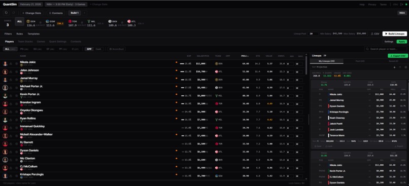
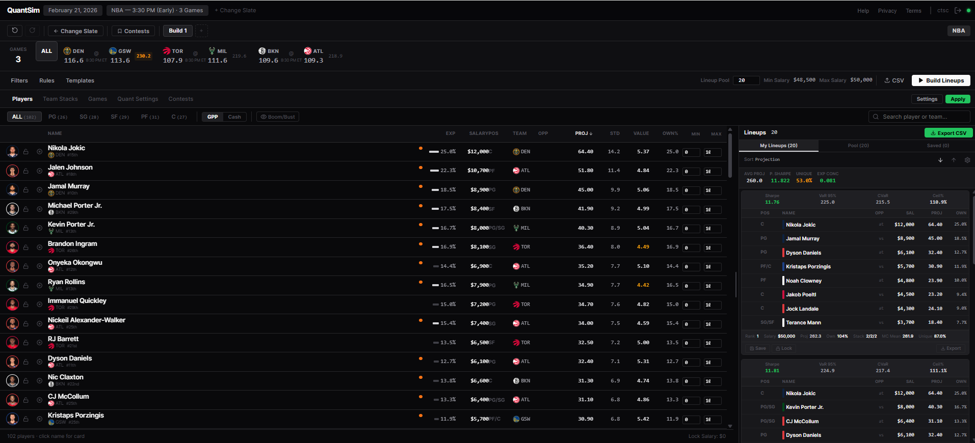
Optimizer Dashboard
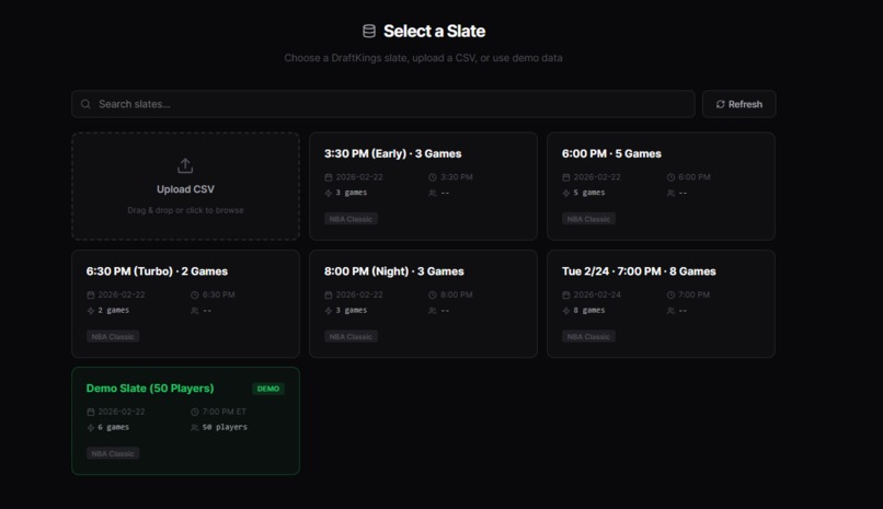
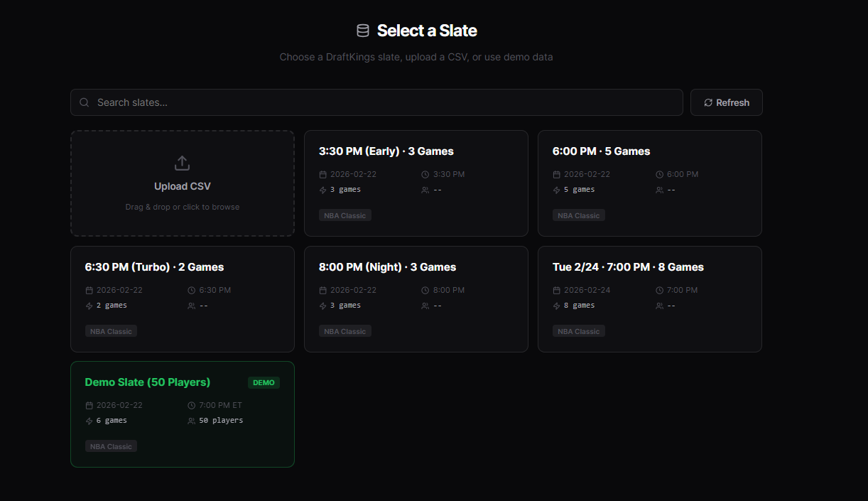
Different Game Slates
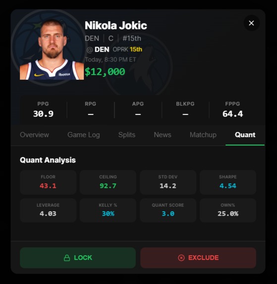
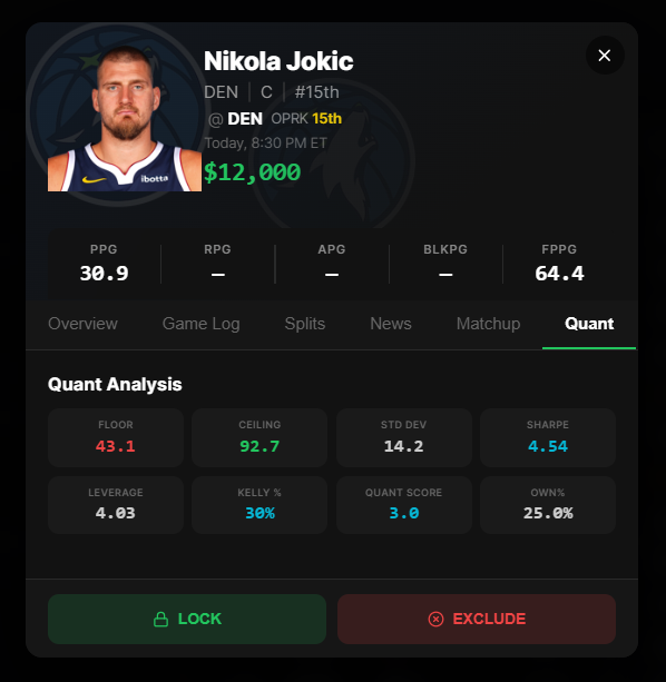
Nikola Jokic
Research Paper
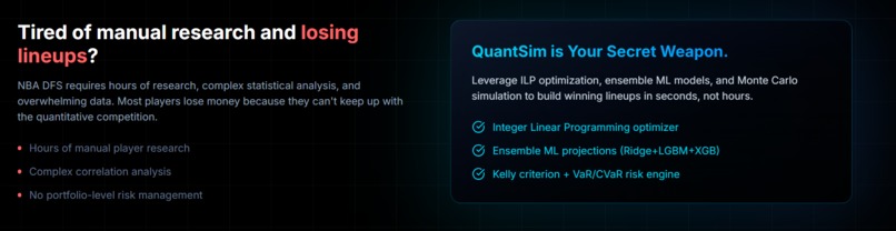
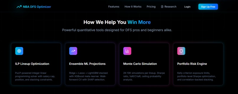
Landing Page
Info
Cool Stuff

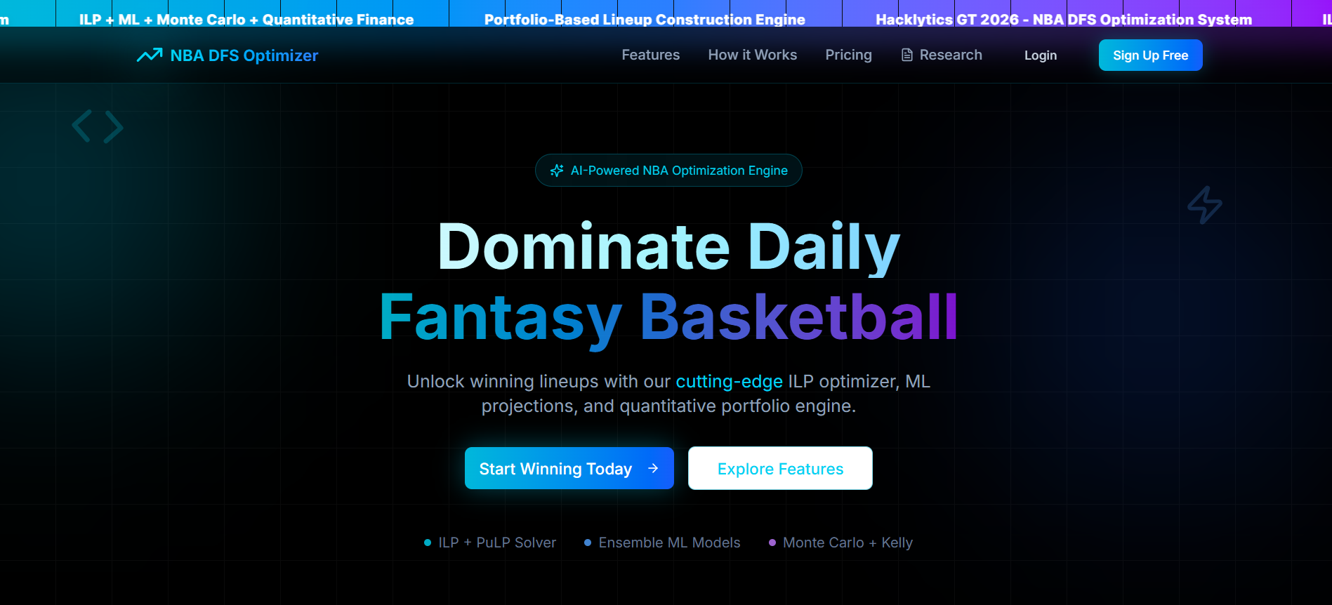
QuantSim: Portfolio-Grade NBA DFS Optimization

The Market

Daily Fantasy Sports (DFS) is a game where you pick a roster of real NBA players — each with a set salary — and score points based on their actual stats that night. The better your lineup, the more you win. It's played on platforms like DraftKings and FanDuel. It is explicitly skill-based and legal in 45 states. And it is enormous: 53 million Americans played fantasy sports in 2024 (FSGA). DraftKings alone generated $5B in revenue in 2024, projecting $6.5–7B in 2025. The global DFS market is $15B and growing at 13.1% annually — on track to hit $50B+ by 2030 (Market Research Future, Mordor Intelligence).

The money is real. DraftKings and FanDuel together control ~67–74% of the US market and have paid out $10B+ cumulatively in prizes. $149.6B was wagered on US sports in 2024 (Legal Sports Report), with 61% of DFS players also sports betting — the highest crossover ever recorded.

Here is the problem: a McKinsey study found that 91% of DFS profits are captured by just 1.3% of players. Three-quarters of all participants lose money. The platform takes ~10% rake on every entry. The only players who win consistently are running analytics — modeling matchups, projecting performance, managing exposure across hundreds of lineups. Professional DFS players treat it as a quantitative operation. The tools that enable this — SaberSim, FantasyLabs, FantasyCruncher — are subscription SaaS products charging $20–$250/month with hundreds of thousands of paying users. QuantSim is our entry into that market.

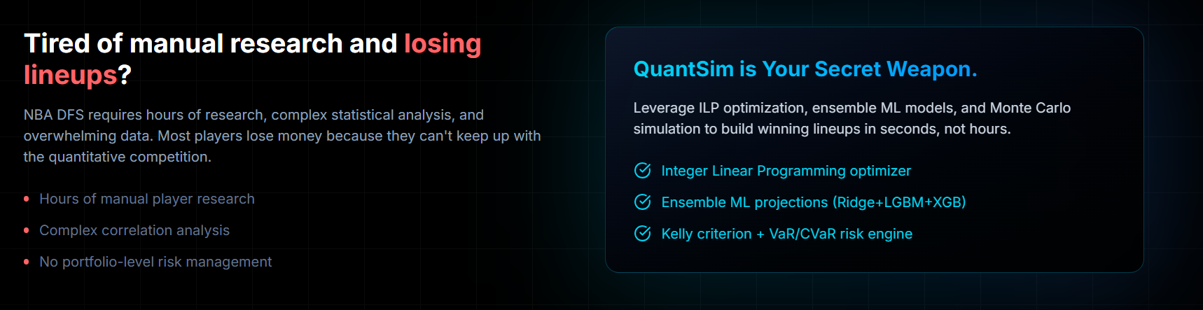
What We Built — And Why It's Better

Our ensemble ML model achieves MAE = 7.37 DraftKings fantasy points on 544,837 player-game observations — matching or beating every benchmark in the published academic literature, and significantly outperforming all commercial DFS projection providers (~8.0 MAE, Döpke et al. 2024). Our system combines this prediction accuracy with end-to-end portfolio optimization. We built the full stack: ML predictions → lineup construction via Integer Linear Programming → Monte Carlo risk evaluation → DraftKings export.

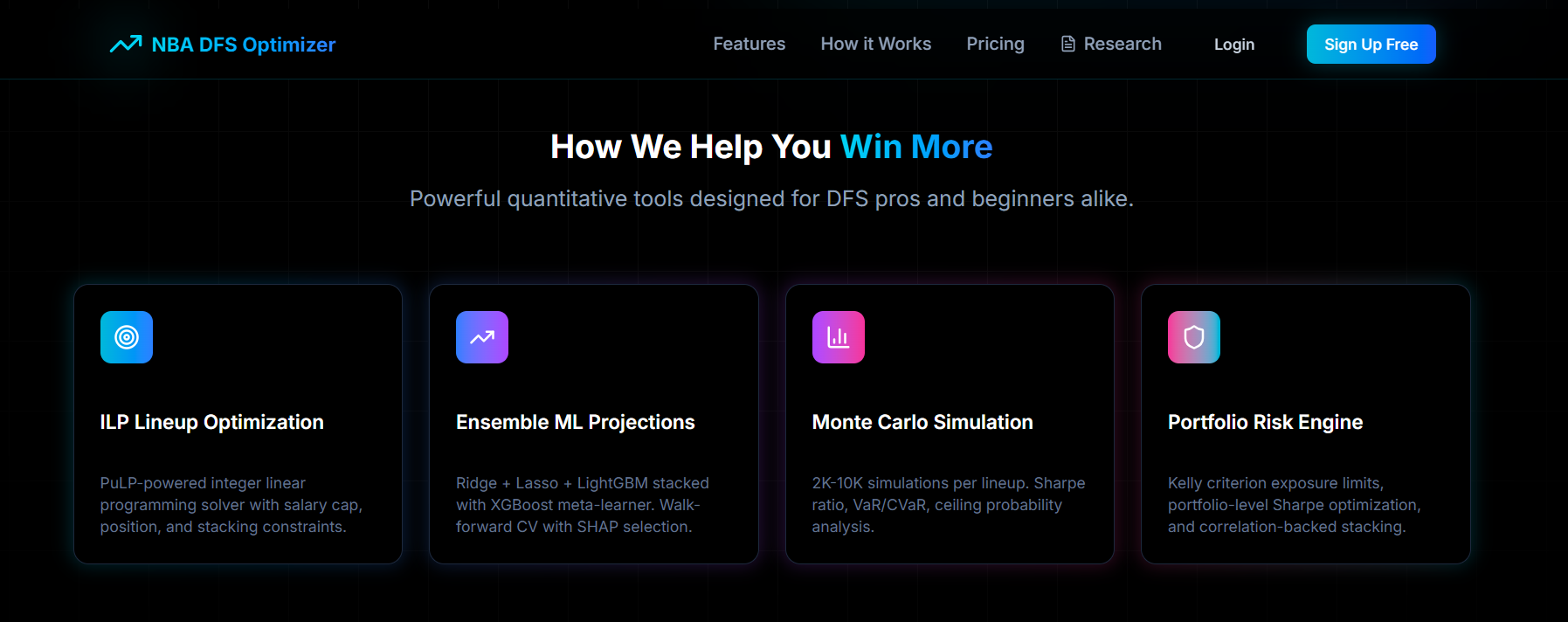
The System (4 Stages)

Stage 1 — Predict

We scraped 21 NBA seasons (2004–2025) of player game logs via nba_api, then trained a stacking ensemble (Ridge + Lasso + LightGBM → XGBoost meta-learner) on 544,837 observations using 128 cores on Modal cloud (~12 minutes total).

Three feature engines generate ~109 strictly pre-game features:

Financial: SMA, EMA, Rate of Change, Bollinger Bands, momentum — applied to each player's DK points time series across 7/14/28-game rolling windows
Probabilistic: rolling volatility (GARCH-inspired), historical VaR, CVaR, and regime detection (hot/cold/neutral states via z-score threshold)
Copula: lagged cross-stat rolling correlations compressed to 8 PCA components — capturing how a player's points, rebounds, and assists co-move

SHAP selects the top 100. Optuna tunes LightGBM hyperparameters over 50 Bayesian trials. Walk-forward CV with a 7-day gap prevents leakage — every fold trains only on data available before that day's games.

Stage 2 — Build

An Integer Linear Program (PuLP + COIN-OR CBC) selects 8 players to maximize projected DraftKings points, subject to: $50K salary cap, position rules (PG/SG/SF/PF/C + G/F flex), per-player exposure limits, lineup diversity constraints, and correlation-backed stacking (PG+C ρ=0.48, game stacks ρ=0.25–0.40).

Stacking is enforced as auxiliary ILP constraints — not projection bonuses — preserving solver optimality. Projections are immutable; modifying them would solve a different problem (Bertsimas & Tsitsiklis, 1997).

Stage 3 — Score

Every lineup runs through 2,000–10,000 Monte Carlo simulations (<500ms). We compute Sharpe ratio, VaR₉₅, CVaR₉₅, ceiling probability, and Kelly-optimal exposure per player. Portfolio metrics (Jaccard uniqueness, Herfindahl concentration index) evaluate the full lineup set — not just individual entries.

Stage 4 — Export

A React + TypeScript web app provides the full interactive interface. Generated lineups export as upload-ready DraftKings CSVs with correct slot mapping (PG/SG/SF/PF/C/G/F/UTIL) — straight to contest entry.

Results

Model Accuracy (Walk-Forward CV, 5 Folds, 7-Day Gap)

FOLD	TRAIN ROWS	MAE ↓	R² ↑
0	89,740	~7.18	0.544
1	179,480	~7.30	0.555
2	269,220	7.215	0.564
3	360,885	7.534	0.573
4	451,518	7.616	0.589
Mean	—	7.37	0.565

R² increases monotonically with data size — the signature of genuine learning.

Walk-forward CV means fold N trains on the first N/5 of chronological game history. Each test window is separated by a 7-day gap to prevent any look-ahead leakage. Fold 0 and 1 MAE values are derived from the reported mean; folds 2–4 are directly measured.

vs. Published Benchmarks

SYSTEM	MAE ↓	SEASONS	OBSERVATIONS	APPROACH
QuantSim (2026)	7.37	21	544,837	Single global stacking ensemble
Papageorgiou et al. (2024)	7.43	10	~40K	203 separate per-player models
Commercial providers (Döpke et al. 2024)	~8.0	1 mo.	1,658	Proprietary

We match the best academic result using a single global model on 13× more data — and significantly outperform the commercial tools people actually pay for. Per-player models (Papageorgiou) can't predict rookies or low-sample players; ours can.

Backtesting (480 Historical Slates)

MODE	CONFIG	RESULT
Cash	30% max exposure, no stack	68.9% cash hit rate (vs. ~50% break-even)
GPP	100% exposure, 3-man stack	85% of hindsight optimal
Portfolio Sharpe	Cash / GPP	1.05 / 0.82

The Stack

LAYER	TECHNOLOGY
Frontend	React 18 + TypeScript + Vite + Radix UI
Backend	Node.js + WebSocket
Optimizer	Python + PuLP + COIN-OR CBC (<100ms/lineup)
ML	scikit-learn + XGBoost + LightGBM + SHAP + Optuna
Volatility	Rolling stddev (GARCH-inspired, via `arch` library fallback)
Cloud training	Modal — 128 cores, parallel walk-forward folds

Challenges

Beating the market — the research burden of actually understanding where commercial tools fail (data leakage, no walk-forward CV) and closing those gaps. The .shift(1) anecdote makes it concrete: forgetting a single lag inflates R² from 0.02–0.15 to ~0.96. That leaked model looks brilliant until it scores 0 in production.

Python ↔ Node boundary — subprocess communication, environment mismatches, Windows/Linux deploy surface, Modal container configuration. JSON contracts at the seam keep it manageable.

Scale exposed shortcuts — rolling group operations on 544K rows, parallel fold execution without shared state. SHAP sampling (50K rows out of 544K) cuts compute from hours to minutes without materially affecting feature selection.

What We Learned

Quantitative finance methods are load-bearing, not decoration. Kelly/VaR/Sharpe applied to DFS lineup construction is novel — no commercial competitor offers it. The portfolio framing changes the optimization question from "what's the best lineup?" to "what's the best set of lineups?", and the backtest Sharpe ratios prove the difference is real.

ML model integrity matters more than architecture. Leakage detection and temporal integrity — using only pre-game features, enforcing .shift(1) everywhere, validating with walk-forward CV — deliver an honest R² of 0.565. A leaked model that scores 0.96 in training is useless in production.

Seam design determines extensibility. JSON contracts at the Python/Node boundary, isolated build state per lineup set, and subprocess lifecycle management make the system composable rather than fragile.

What's Next

Ownership projection model — ML-based ownership% predictions for GPP leverage scoring
Field simulation — ownership-weighted contest field → true ROI estimates
Multi-sport extension — NFL and MLB using the same pipeline architecture

Longer term: Kelly-based bankroll sizing and multi-contest entry allocation across different contest types (cash vs. GPP vs. satellite).

The 1.3% of DFS players who win consistently already run analytics. We built the system that lets anyone play like they do — with the math to prove it works.