PulmoScan

Home Page
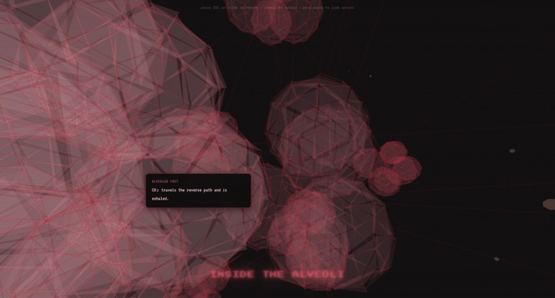
Alveoli Dive
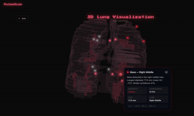
3D Lung
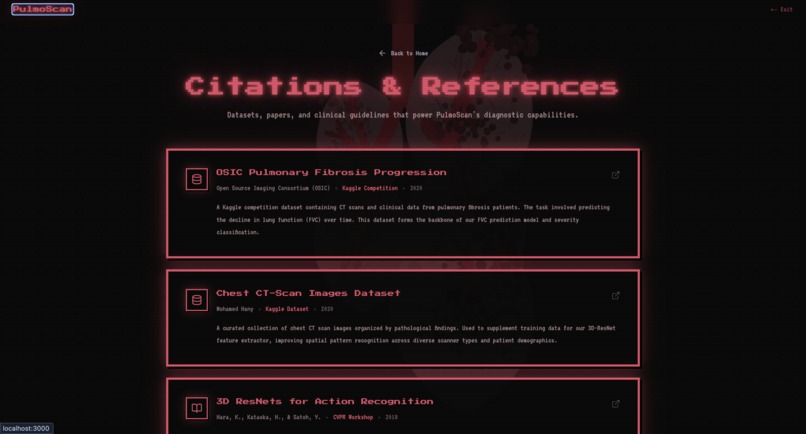
Citations Page

Inspiration

Every 26 minutes, a Canadian dies from lung cancer. It remains the country's deadliest cancer — responsible for more deaths annually than breast, colorectal, and prostate cancers combined — yet survival rates have barely improved in two decades because the disease is overwhelmingly caught too late. By the time symptoms surface, the cancer has often metastasized beyond the lung.

This project is personal. One of our teammate's grandmothers underwent a routine chest CT after persistent coughing that her family assumed was seasonal. The scan revealed a 14mm nodule in her right upper lobe — but the referral to a pulmonologist took eleven weeks. By the time she was seen, what could have been a Stage Ib adenocarcinoma had progressed to Stage IIIa with lymph node involvement. The gap wasn't in the scanning — it was in the interpretation and urgency. The CT data existed. The insight was buried inside 247 grayscale slices that sat in a queue.

That experience exposed a systemic failure: radiologists processing lung CTs are performing an extraordinary cognitive task — mentally reconstructing three-dimensional anatomy from hundreds of flat, 2D images and spotting millimeter-scale anomalies within them. Studies show that 20–30% of actionable nodules are missed on initial reads due to this cognitive burden, and the median wait time for specialist follow-up in Canada's public system exceeds 8 weeks. The data is there. The diagnosis is trapped inside it.

We built PulmoScan to break it out — to take raw CT data and transform it into something a clinician can see, rotate, fly through, and immediately understand, with AI highlighting exactly where the problem is and how severe it looks.

What It Does

PulmoScan takes a patient's raw DICOM CT scan series — a folder of ~200 sequential cross-sectional images — and runs it through a fully automated pipeline that produces four outputs in a single pass:

3D Volume Reconstruction: The DICOM slices are loaded, calibrated to Hounsfield Units, resampled to isotropic 1mm³ spacing, and stacked into a true volumetric dataset. Flat images become spatial anatomy.

Lung Segmentation: The lung parenchyma is isolated from surrounding tissue (ribcage, mediastinum, body wall) using an Otsu thresholding and morphological cleanup pipeline, producing a labeled volume where left and right lungs are individually identified.

AI-Powered Pathology Detection: A dual-track detection system — one rule-based, one deep learning — scans the segmented lung for anomalous regions. Each finding is classified by type (nodule, mass, ground-glass opacity, consolidation), localized to a specific lobe, measured in millimeters, and assigned a severity score and confidence rating. Grad-CAM heatmaps provide visual evidence of where the model sees pathology.

Interactive 3D Visualization: The segmented lung renders in-browser as a translucent, glass-like holographic structure using VTK.js with marching cubes surface extraction. Detected pathology appears as coral-pink glowing masses floating inside the lung volume. Users can rotate 360°, zoom, drag a cross-section blade through the model, and click any finding to fly the camera directly to it. Annotation dots float in 3D space next to each finding, showing its label and severity.

The result: a clinician uploads a scan and within 30 seconds has an interactive, explorable 3D model of the patient's lungs with every detected anomaly highlighted, measured, and classified — eliminating the cognitive translation from 2D slices to 3D anatomy entirely.

How We Built It

PulmoScan is architected as three independent layers — an ML pipeline, a 3D rendering engine, and a frontend application — all communicating through a shared JSON contract schema that was defined before any code was written. This allowed three developers to build in parallel with zero merge conflicts across the entire hackathon.

ML Pipeline (⁠ /ml ⁠)

The ML layer handles everything from raw DICOM bytes to exportable 3D volumes and clinical findings.

DICOM Loading (⁠ dicom_loader.py ⁠): CT series from the OSIC Pulmonary Fibrosis Progression dataset are loaded using SimpleITK. Each patient's folder contains ~100–400 ⁠ .dcm ⁠ files representing sequential axial slices. The loader reads the full series, extracts spatial metadata (origin, spacing, direction cosines) from DICOM headers, and produces a 3D NumPy array in Hounsfield Units. Voxel spacing varies across scanners (typically 0.6–0.8mm in-plane, 1.0–2.5mm slice thickness), so the volume is resampled to isotropic 1mm × 1mm × 1mm resolution using ⁠ scipy.ndimage.zoom ⁠ with spline interpolation of order 1 — normalizing cross-scanner variance so downstream algorithms operate on a consistent spatial grid.

Lung Segmentation (⁠ segmentation.py ⁠): Implements a multi-stage morphological pipeline: 1.⁠ ⁠Otsu thresholding separates air-density voxels (lung parenchyma, ~−700 HU) from soft tissue and bone 2.⁠ ⁠Border-connected components are cleared to remove extracorporeal air 3.⁠ ⁠3D connected component labeling identifies discrete regions; the two largest are retained as left and right lung 4.⁠ ⁠Morphological closing with a ball structuring element (radius 3–5 voxels) smooths the lung boundary to prevent jagged marching cubes surfaces 5.⁠ ⁠The output is an ⁠ int32 ⁠ label map: 0 = background, 1 = left lung, 2 = right lung

Pathology Detection (⁠ pathology.py ⁠): Runs a dual-track system for maximum coverage:

Track A (Rule-Based): Within the lung mask, connected components with mean HU exceeding −400 (indicating solid tissue where there should be air) are extracted, filtered by equivalent diameter (≥ 3mm), and classified by HU statistics: ground-glass opacity (−600 to −400 HU), consolidation (−100 to +100 HU), solid nodule/mass (mixed density). Each component's centroid is converted from voxel to world coordinates using ⁠ center_world = center_ijk × spacing + origin ⁠, and severity is assigned by Fleischner Society size criteria: < 4mm = low, 4–8mm = moderate, 8–20mm = high, > 20mm = critical.

Track B (Deep Learning): An EfficientNet-B0 classifier — pretrained on ImageNet (1.4M images, 1000 classes) with a custom head: ⁠ AdaptiveAvgPool2d → Dropout(0.3) → Linear(1280, 4) ⁠ — is trained on the Chest CT-Scan Images dataset (~1000 labeled PNGs across 4 classes: adenocarcinoma, large cell carcinoma, squamous cell carcinoma, normal). Training uses AdamW optimizer at $lr = 1 \times 10^{-3}$ with cosine annealing over 20 epochs on MPS (Apple Silicon GPU). The training folder names encode clinical metadata (e.g., ⁠ adenocarcinoma_left.lower.lobe_T2_N0_M0_Ib ⁠), which is parsed to extract lobe location and TNM staging. Grad-CAM targets the final convolutional block of EfficientNet-B0, backpropagating gradients from the classification output to produce spatial heatmaps that highlight the image regions driving the prediction. Track B runs with a 60-second timeout and falls back to Track A if it exceeds the limit.

Export: Three NRRD volumes are generated per scan using ⁠ pynrrd ⁠ with gzip encoding: ⁠ ct_volume.nrrd ⁠ (the resampled CT), ⁠ lung_segmentation.nrrd ⁠ (the lung label map), and ⁠ pathology_mask.nrrd ⁠ (the pathology label map). All carry correct ⁠ space directions ⁠ (diagonal matrix from spacing) and ⁠ space origin ⁠ (from DICOM ⁠ ImagePositionPatient ⁠) headers — these are critical because the VTK.js viewer reads them to position the 3D model at the correct scale and orientation. A ⁠ scan_result.json ⁠ conforming to the contract schema accompanies the volumes, containing patient metadata, finding details, and volume URLs.

Backend (⁠ /backend ⁠)

FastAPI serves as the API layer between the frontend and the ML pipeline:

•⁠ ⁠⁠ POST /api/analyze ⁠ accepts a ⁠ patient_id ⁠ (form field) or an uploaded DICOM zip, invokes ⁠ pipeline.py ⁠, and returns the contract JSON with volume URLs pointing to ⁠ /assets/ ⁠ •⁠ ⁠⁠ GET /api/patients ⁠ scans the ⁠ data/osic/train/ ⁠ directory and returns available patient IDs with slice counts •⁠ ⁠⁠ GET /api/health ⁠ reports server status and model availability •⁠ ⁠⁠ /assets/ ⁠ serves generated NRRD and JSON files as static content •⁠ ⁠CORS is configured for the frontend's development port

3D Viewer (⁠ /frontend/viewer ⁠)

The visualization engine runs entirely in the browser using ⁠ @kitware/vtk.js ⁠, a WebGL-based medical imaging library developed by Kitware.

Surface Extraction: ⁠ vtkImageMarchingCubes ⁠ processes each 3D label map at contour value 0.5, generating triangle meshes at the boundary between labeled and unlabeled voxels. Two marching cubes instances run in parallel — one for the lung surface, one for pathology.

Translucent "Glass" Lung: The lung mesh renders with ⁠ vtkActor ⁠ properties calibrated for a holographic effect: ⁠ opacity: 0.15–0.25 ⁠, ice-blue coloring ⁠ [0.65, 0.82, 0.92] ⁠, high specular reflection (⁠ specular: 0.9 ⁠, ⁠ specularPower: 60 ⁠), and ⁠ backfaceCulling: false ⁠ so interior surfaces remain visible when the model is clipped.

"Lava" Pathology: Pathology surfaces render as opaque coral-pink masses (⁠ opacity: 1.0 ⁠, ⁠ color: [0.95, 0.45, 0.42] ⁠) with elevated specular intensity, creating an immediate contrast against the surrounding translucent lung tissue.

Interaction: ⁠ vtkInteractorStyleTrackballCamera ⁠ provides native 360° rotation and scroll-to-zoom. Clickable annotation dots are positioned using ⁠ vtkCoordinate ⁠ world-to-display projection, updated on every camera change. Clicking a dot or a sidebar finding triggers an animated camera ⁠ flyTo ⁠ using ⁠ requestAnimationFrame ⁠ interpolation to the finding's ⁠ center_world ⁠ coordinates.

Frontend (⁠ /frontend ⁠)

Built with Next.js 14, TypeScript, Tailwind CSS, and Framer Motion.

The landing page introduces the platform with a cinematic hero section and animated feature breakdown. The scanner page presents available OSIC patients in a selectable grid; on selection, a processing animation with cycling medical status messages covers the 10–30 second pipeline execution. The dashboard implements a split-panel layout: a scrollable findings sidebar on the left (with severity badges, confidence bars, lobe labels, and millimeter measurements) and the 3D viewport filling the remaining space. A bidirectional state flow connects them: clicking a finding in the sidebar sets ⁠ activeFindingId ⁠ which triggers camera flyTo in the viewer, while hovering pathology in the 3D scene fires ⁠ onFindingHover ⁠ which highlights the corresponding sidebar card — creating a unified interaction where 2D clicks navigate in 3D space and 3D hovers highlight in 2D.

Challenges We Ran Into

Bridging 2D classification with 3D visualization was our most complex architectural decision. Our cancer classifier trains on isolated 2D PNG slices (Chest CT-Scan Images dataset), while the 3D viewer requires complete volumetric DICOM series (OSIC dataset). These are fundamentally different data — one is a single image from an unknown patient, the other is a full spatial scan from a specific patient. We solved this by running both tracks in the pathology detection phase: Track A operates directly on the 3D volume to find anomalies spatially, while Track B classifies extracted slices and maps the predicted lobe back to 3D coordinates. The dual-track approach means we catch findings that either method alone would miss.

Coordinate system consistency nearly broke the pipeline. DICOM stores spatial metadata as ⁠ (x, y, z) ⁠, but SimpleITK's ⁠ GetArrayFromImage ⁠ returns arrays in ⁠ (z, y, x) ⁠ order. A single axis transposition error caused lungs to render as flat disks or vertical needles in the viewer. We resolved this by enforcing a strict convention: NRRD headers always carry ⁠ (x, y, z) ⁠ spacing via the ⁠ space directions ⁠ diagonal matrix, ⁠ center_world ⁠ in the findings JSON uses the same coordinate system, and every axis transformation is explicitly documented at the function boundary. The 3D viewer reads these headers directly — if they're wrong, the lung is wrong.

Marching cubes threshold tuning consumed hours of debugging. Label maps use integer values (0 = background, 1 = tissue), and the intuitive contour value of 1.0 produces an empty render. The correct value is 0.5 — the midpoint where the algorithm detects the 0→1 boundary. We traced "blank screen" bugs through the entire NRRD export pipeline before discovering the issue was a single parameter in VTK.js.

Segmentation quality versus processing time forced a direct trade-off. A full watershed segmentation with Sobel edge detection and black-top-hat morphological refinement produces beautifully smooth lung boundaries but takes 60–90 seconds per patient on CPU. The simpler Otsu + morphological closing pipeline completes in 5–8 seconds with slightly rougher boundaries. For a hackathon demo where responsiveness matters, we chose the faster approach and tuned the morphological closing kernel to minimize surface artifacts in the marching cubes output.

Accomplishments That We're Proud Of

We built a complete, end-to-end medical imaging pipeline — from raw DICOM bytes to an interactive 3D lung model with AI-classified pathology glowing inside it — in under 24 hours with a team of three. The system processes real patient CT data from the OSIC dataset, not synthetic test models, producing anatomically accurate 3D reconstructions that faithfully represent the scanned patient's lung geometry.

The three-person parallel development workflow — where ML, 3D viewer, and frontend were built simultaneously in separate directories against a shared JSON contract — resulted in zero merge conflicts across the entire hackathon. Integration required mounting one React component and pointing one environment variable at the backend URL. The contract-first architecture proved that three people can build a complex, tightly coupled system without ever touching each other's code.

The dual-track pathology detection system combining classical computer vision (HU thresholding + connected components) with deep learning (EfficientNet-B0 + Grad-CAM) provides both spatial precision on 3D volumes and classification confidence on 2D slices — covering cases that either approach alone would miss.

Most importantly, this project was built to honor a real person whose diagnosis came too late because the data was there but the insight wasn't. If PulmoScan can compress the time between "scan acquired" and "findings understood" from weeks to seconds, that's the gap we exist to close.

What We Learned

A CT scan is not an image. It is a calibrated, three-dimensional measurement of physical density at every point inside a human body, expressed in Hounsfield Units where air is −1000, water is 0, and bone is +1000. Understanding this changed how we approached every stage of the pipeline — segmentation thresholds are not arbitrary numbers but physical density boundaries between tissue types, and resampling to isotropic spacing is not a preprocessing convenience but a requirement for spatially consistent 3D analysis.

We also learned that the distance between "technically correct" and "clinically intuitive" is where the actual product lives. A raw marching cubes mesh of a segmented lung is geometrically accurate but visually meaningless — it looks like a grey blob. Adding translucency, specular lighting, pathology glow, camera animation, and cross-section interaction transforms identical data into something a clinician can immediately parse. The rendering is not cosmetic — it is the interface between computational output and human spatial reasoning, and it is the reason this project exists.

Finally, we learned that in medical AI, the model is the easy part. The hard part is everything around it: loading heterogeneous DICOM files from different scanners with different spacings and orientations, preserving coordinate systems through four layers of transformation, ensuring that the millimeter coordinate where the AI says "nodule" is the same millimeter coordinate where the 3D camera flies to. The infrastructure of correctness is harder than the inference.

What's Next for PulmoScan

Our first priority is replacing the Otsu-based segmentation with a pretrained 3D U-Net (such as those from the Medical Segmentation Decathlon) for faster, more robust lung boundary extraction that handles edge cases like severe fibrosis, pleural effusion, and post-surgical anatomy where simple thresholding fails.

On the detection side, we plan to train a 3D convolutional network directly on volumetric DICOM data rather than classifying extracted 2D slices — enabling the model to learn spatial patterns (spiculation, ground-glass halos, calcification patterns) that are invisible on any single cross-section.

For clinical deployment, we aim to integrate with hospital PACS (Picture Archiving and Communication Systems) via DICOMweb so clinicians can pull patient scans directly into PulmoScan without manual file transfers. We also plan to add longitudinal tracking — overlaying scans from different dates to measure nodule growth velocity, which is the clinical gold standard for determining whether a finding requires biopsy.

On the rendering side, we want to implement level-of-detail switching in VTK.js (coarse mesh during rotation, full resolution when stationary) and move NRRD decompression into a Web Worker to bring the initial 3D load time under 3 seconds on standard hardware.

Above all, we want to close the gap that cost our teammate's grandmother critical months — the gap between "data acquired" and "findings understood." Every week a diagnosis sits in a radiologist's queue is a week the disease progresses. PulmoScan's mission is to make that wait time zero.