Predicting Pipe Flow With Neural Networks

Poster!

Final Checkin and Project Report: link

11/28 Checkin: link

Title: Deep Learning to Solve Physical Problems Faster

Names and Logins: Alexander Koh-Bell (akohbell), Jason Gong (jgong15), Joshua Neronha (jneronha)

Introduction

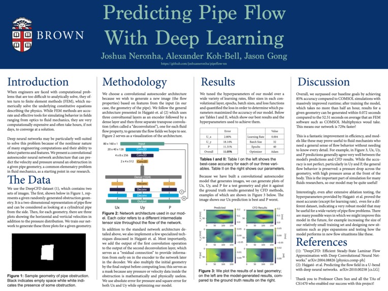
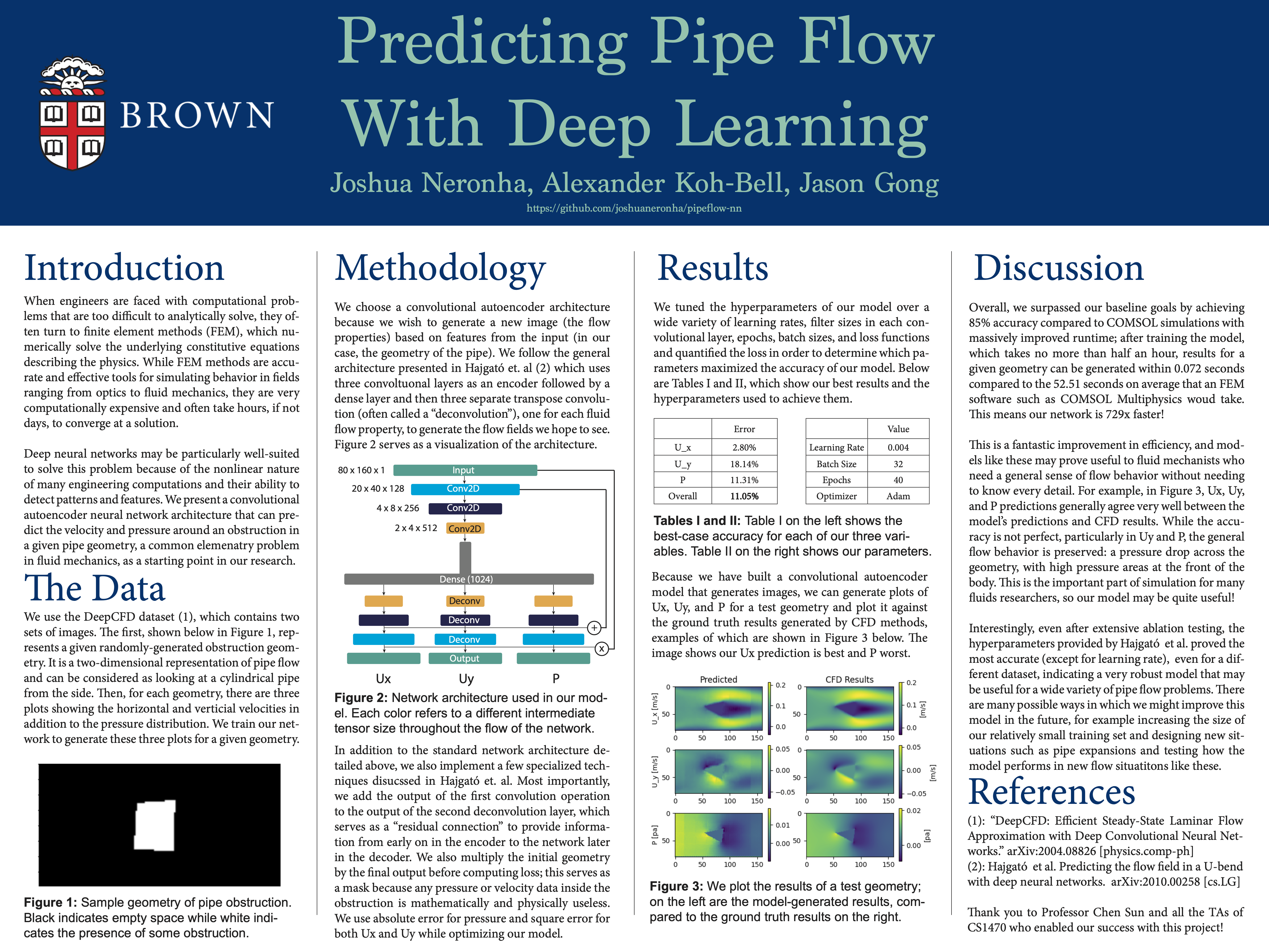
When engineers are faced with computational problems that are too difficult to analytically solve (which is usually the case), they often turn to finite element methods (FEM), which numerically solve the underlying constitutive equations describing the physics. While FEM methods are extraordinarily accurate and effective tools for simulating behavior in a variety of fields ranging from optics to fluid mechanics, they are very computationally expensive and often take hours, if not days, to converge at a solution because of the fine meshing required to obtain an accurate solution. As a group partially composed of mechanical engineers, we are very familiar with how slow FEM can be; it is not uncommon to spend over a day waiting for results before realizing a small parameter was not properly set, requiring even more time to get results. We believe that artificial deep neural networks may be particularly well-suited to solve this problem because of the nonlinear nature of many engineering computations and their ability to detect patterns and features. There are many areas within physics and engineering that we could focus on, but we have chosen to focus on pipe flow, a situation often considered by civil or mechanical engineers in a wide variety of contexts. This is because pipe flow in a cylindrical pipe is a fairly simple problem to solve, making it a good starting point. However, it is easy to add complexity, whether that be varying the shape of the pipe’s cross-section, adding obstructions, or rapidly expanding or compressing the flow in the pipe, which is good for our project. We expect this to be a regression-based problem that aims to solve for the pressure and velocity at a variety of locations in the pipe.

Related Work

There is a wealth of prior research on applications of deep learning to physics problems, including quite a bit at Brown! Prof. George Karniadakis in Brown’s Applied Math department developed a deep-learning technique called physics-informed neural networks that essentially impose constraints on deep learning models based on the constitutive laws of physics. While interesting, we wish to solve problems entirely using deep learning methods without having to specify the underlying physics in hopes that the model is able to “learn” the laws of physics similar to how we as humans have physical intuition as to their effects from an early age. As a result, we will focus on entirely deep-learning based methods. One paper that serves as inspiration for our project and will be very useful when developing the architecture is a 2018 article by Hajgató et. al at the Budapest University of Technology and Economics titled "Predicting the flow field in a U-bend with deep neural networks.” In the paper, the authors attempt to use a combination of convolutional neural networks (CNNs) with autoencoders in order to predict the velocity field. The idea is to pass in an image representing the shape of the pipe, use a convolutional neural network to learn features of the pipe’s design, then use autoencoders to predict the velocity field. Because there is very little computational fluid dynamics (CFD) data published on the Internet, the authors generated their own data using CFD software. Using a GPU, the authors were able to simulate results using the neural network architecture with very similar accuracy to the CFD model (an average difference of 0.009 m/s) at up to 1500x faster! As a result, this is a very promising model for predicting pipe flow that we will use as inspiration and reference for our own deep learning model. While we will be using this paper as the basis for our architecture we are not really just re-implementing it for a few reasons because neither the data or code is provided -- we will be writing our model from scratch and obtaining data from another source. We also will solve a different problem than a U-shaped pipe -- we will instead aim to understand the flow field as a function of randomly shaped obstructions. Thus, while making reference to prior architectures, this will in effect be new research using an existing architecture as a starting point.

Data

We originally planned to generate our own data, but found access to CFD software more challenging than expected. As a result, we are using the DeepCFD project's data repository, which provides flow results of velocity and pressure for various obstructions in a two-dimensional pipe geometry!

Methodology

Our project will use a neural network for the purpose of modeling predicting the velocity file of a fluid through a pipe. The project will implement convolution for the purpose of interpreting inputs as well; this will make it so that the model will express translational invariance and thus not be sensitive to the placement of the same image of a given pipe. As a result, the first step of our architecture will be convolutions to detect features of the pipe shape given black and white images of the pipe’s shape. Then, we will implement an encoder/decoder model using deconvolutional layers, as detailed in the referenced paper on which we will be basing our architecture. We plan to follow the paper’s architecture as a guide but may modify it slightly based on our own needs and what we find to work best for our specific project.

To test our model, we will use a testing set of data that shows the flow results for a given geometry. We will randomly take a percentage of our input data as testing data and exclude it from the training set. We will then calculate accuracy in testing, and average accuracy will be a metric of success. For the case of a pipe flow speed distribution, we will discretize and represent this distribution as a vector of velocities at each incremental point in the flow. These vectors outputted by the model will be compared with that of testing data by calculating the difference between the vectors, which can be used to define accuracy.

Metrics

To test our model, we will use a testing set of data. We will randomly take a percentage of our input data as testing data and exclude it from the training set. We will then calculate accuracy in testing, and average accuracy will be a metric of success. For the case of a pipe flow speed distribution, we will discretize and represent this distribution as a vector of velocities at each incremental point in the flow. These vectors outputted by the model will be compared with that of testing data by calculating the difference between the vectors, which can be used to define accuracy.

Our general goal is to make a deep learning model that can make accurate calculations for physical problems, all while doing this faster than physics-based simulations (not including training time). Our base goal is to have a model with an accuracy of greater than 80%, and a lower time per calculation than the COMSOL physics simulations. Our target goal is to have a model with accuracy greater than 95% that runs 5x faster than COMSOL simulations. Our stretch goal will be to create a model that can meet these criteria (95% accuracy, 5x faster than COMSOL) for more than one particular type of physical problem. This could include meeting these criteria for our original pipe flow problem as well as for a turbulent or viscous pipe flow problem. Additional goals will include fine tuning our model such that accuracy and speed are high while required sample size of input data is low.

Ethics

The broader issue of energy consumption and related climate change is very relevant to our chosen problem. The idea of training a deep learning algorithm to perform physical simulations faster and with fewer computations than existing simulations can in some ways reduce energy consumption. If users replaced their day to day physical simulations with a computationally faster deep learning model, they would be using less computational power and thus energy, although training the model would require additional electrical power. However, most of the exciting applications of this kind of model that can solve physical problems very quickly involve making large numbers of calculations, which will require electrical power. Example applications include making continuous real-time physically realistic animations for creative or video-game purposes, or running an optimization algorithm on design parameters using this kind of deep learning algorithm to evaluate the function at each point. Both of these applications are often unrealistic with typical physical simulations, because they require large numbers of computations, but they would be possible with such a faster model. Based on these applications, this field of deep learning is likely to overall contribute to increased electricity consumption from these kinds of physical calculations. On the other hand, these potential applications do have significant societal benefits. For example, enabling computational design optimization of renewable energy technology or energy efficient vehicles is beneficial for the environment. Taking this example application, the stakeholders are the direct users of the algorithms and those who use or benefit from designs that were informed in part by this algorithm. Some may argue that increased capability of computational design optimization will take away jobs from design engineers who currently or previously would make these designs themselves. While I have not analyzed evidence for this, it is also likely that these engineering stakeholders would still be employed, since they would typically be assigned to using these kinds of algorithms and assuring quality. A main danger of mistakes in the algorithm would be the impact on the end users of a product that was informed by these simulations. Taking the electric vehicle example, errors in the computation based design process could lead to accidents and damage to the drivers/passengers. However, realistically, this kind of deep learning model would be used as an approximation to simulations that is used in the optimization process, and an ‘optimized’ design would then be verified/simulated using standard/slower physics based simulations, as well as human experts. In this example though, mistakes in the algorithm could realistically lead to the optimization algorithm outputting an incorrect ‘optimum’, as a true global optimum may have been missed due to an error, which would lead to the electric vehicle potentially being less efficient than it would have been, resulting in higher energy consumption.

Division of Labor

We all plan to contribute to all aspects of this project. Josh will lead the task of gathering and processing data for training and testing, Jason will focus more so on the deep learning model itself, and Alex will also largely focus on the deep learning model but assist with data generation and integration. (subject to change!)