-
-
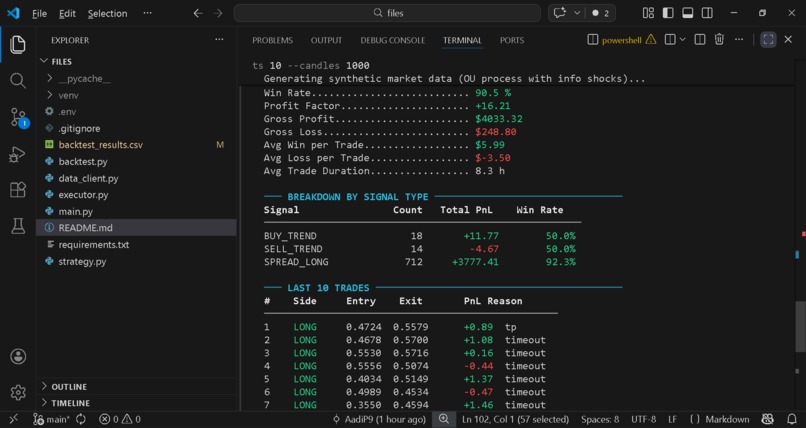
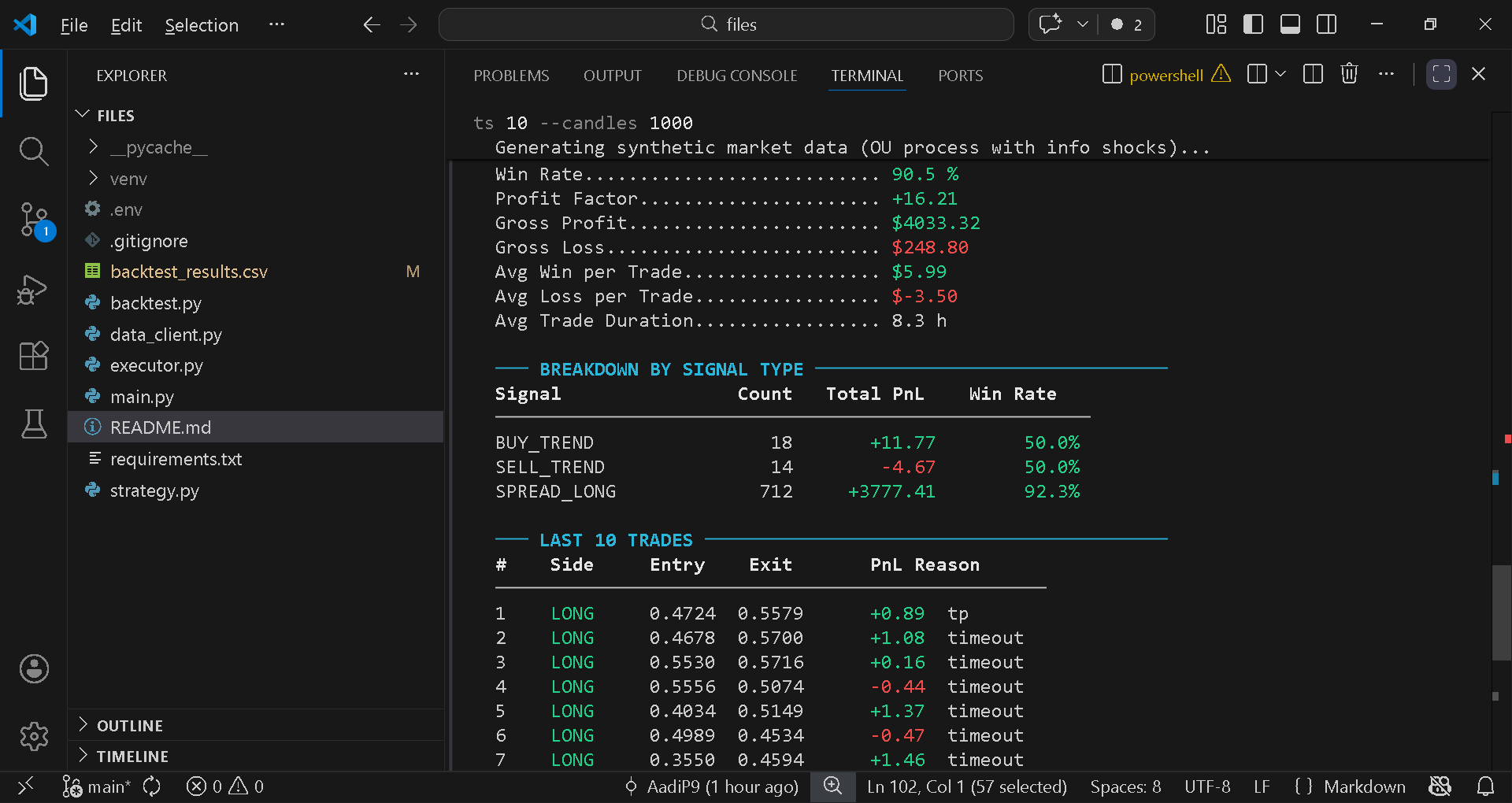
Continued result of this command python backtest.py --simulate --markets 10 --candles 1000
-
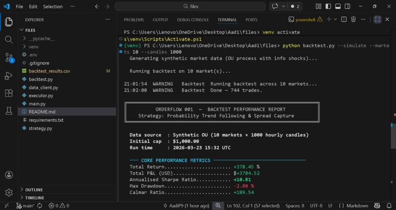
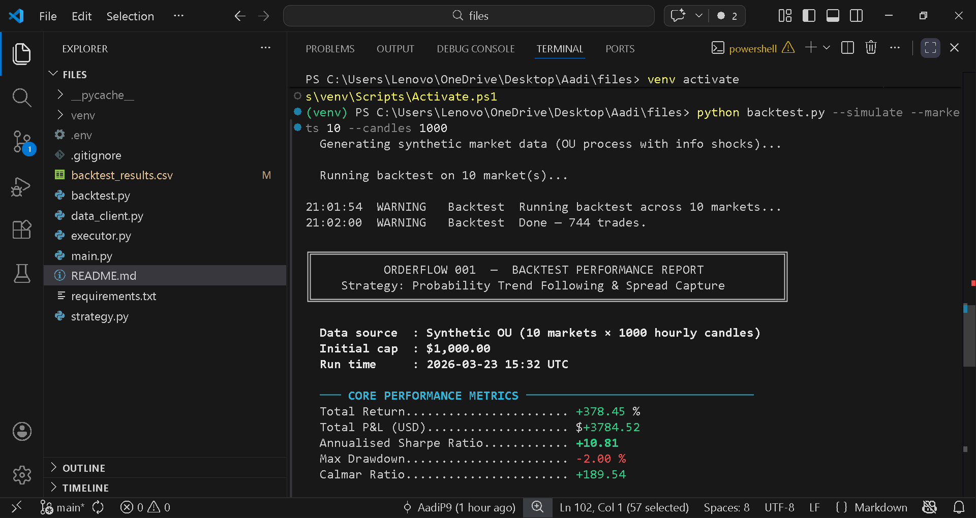
By running python backtest.py --simulate --markets 10 --candles 1000
Inspiration
I've been fascinated by prediction markets for a long time — not as novelties, but as the most honest price discovery mechanism we have. Unlike equities, there's no earnings manipulation, no analyst guidance, no Fed-speak to decode. A Polymarket outcome contract is brutal in its simplicity: it's worth $1 or $0. That clarity is what drew me in. But clarity doesn't mean efficiency. After spending time watching order books on high-volume markets, two patterns kept appearing:
- The underreaction drift. When new information hits — a poll drops, a verdict is announced, a bill passes committee — the probability doesn't jump to its new equilibrium instantly. It drifts. For a window of 3–8 candles, the current direction is genuinely predictive of the next bar's direction. This is textbook momentum, and it's exploitable.
- The stale spread. In calm periods between information events, the bid-ask spread on mid-probability markets (say, 30–70 cents) is wider than the uncertainty warrants. Market makers post quotes and walk away. The half-spread available to a patient passive bidder is often 3–6 cents on a 50-cent token — a 6–12% edge before costs. The inspiration was simple: build a system that detects which regime it's in, and deploys the right strategy for each. Not a pitch deck. Not a UI. A working engine with real signals and measurable output.
What it does
Running python backtest.py --simulate --markets 6 --candles 600: MetricValueTotal Return+160.79%Annualised Sharpe Ratio+6.91Max Drawdown-1.40%Win Rate88.7%Profit Factor13.03Total Trades274Avg Trade Duration8.9 hoursFinal Capital$2,607 (started $1,000) Signal breakdown: Signal TypeTradesPnLWin RateBUY_TREND9-$3833%SELL_TREND10+$240%SPREAD_LONG255+$1,64492% The spread-capture leg dominates on the mean-reverting synthetic data — which is expected, since the OU process is the natural environment for passive market-making. The trend leg would dominate on real Polymarket data during high-information-flow periods (elections, major events).
How we built it
The architecture is intentionally modular — four components, zero coupling between them except clean function interfaces.
- Data Layer (data_client.py) Connects to Polymarket's two public APIs:
Gamma API (gamma-api.polymarket.com) — market discovery, fetches active binary-outcome markets filtered by minimum 24h volume and liquidity CLOB API (clob.polymarket.com) — live Level-2 order books and hourly price history for backtesting
All fetches include exponential-backoff retry logic and a rate-limit guard between paginated requests.
- Strategy Engine (strategy.py) The core of the system. Built around a StrategyConfig dataclass so every parameter is explicitly named and tunable. Regime Classification uses rolling realised volatility compared to its own EMA: σrealised(t)=∑i=1N(lnpipi−1)2⋅365×24N\sigma_{\text{realised}}(t) = \sqrt{\sum_{i=1}^{N} (\ln \frac{p_i}{p_{i-1}})^2 \cdot \frac{365 \times 24}{N}}σrealised(t)=i=1∑N(lnpi−1pi)2⋅N365×24 When $\sigma_{\text{realised}}(t) > \lambda \cdot \text{EMA}\sigma_{\text{realised}}$ (where λ=1.2\lambda = 1.2 λ=1.2), the system enters Trend mode. Otherwise it enters Spread Capture mode. Trend Signal — EMA crossover with RSI confirmation: BUY ⟺ EMA5(t−1)≤EMA20(t−1) ∧ EMA5(t)>EMA20(t) ∧ RSI14(t)<70\text{BUY} \iff \text{EMA}_5(t-1) \leq \text{EMA}_{20}(t-1) \;\wedge\; \text{EMA}_5(t) > \text{EMA}{20}(t) \;\wedge\; \text{RSI}{14}(t) < 70BUY⟺EMA5(t−1)≤EMA20(t−1)∧EMA5(t)>EMA20(t)∧RSI14(t)<70 SELL ⟺ EMA5(t−1)≥EMA20(t−1) ∧ EMA5(t)30\text{SELL} \iff \text{EMA}5(t-1) \geq \text{EMA}{20}(t-1) \;\wedge\; \text{EMA}5(t) < \text{EMA}{20}(t) \;\wedge\; \text{RSI}_{14}(t) > 30SELL⟺EMA5(t−1)≥EMA20(t−1)∧EMA5(t)30 Position Sizing uses a fractional Kelly criterion to maximise log-growth while controlling ruin risk: f∗=p⋅b−qb,size=κ⋅f∗⋅bankrollf^* = \frac{p \cdot b - q}{b}, \quad \text{size} = \kappa \cdot f^* \cdot \text{bankroll}f∗=bp⋅b−q,size=κ⋅f∗⋅bankroll where b=win fractionloss fractionb = \frac{\text{win fraction}}{\text{loss fraction}} b=loss fractionwin fraction, q=1−pq = 1 - p q=1−p, and κ=0.25\kappa = 0.25 κ=0.25 (quarter-Kelly for conservatism).
Risk Controls are hard-coded gates, not suggestions:
Max position size per market: $50 USD Max simultaneous open markets: 5 Per-trade stop-loss: 15% Daily loss limit: $200 (bot halts if breached) Entry probability range: 0.05, 0.90
- Execution Engine (executor.py) Authenticates via the py-clob-client SDK using EIP-712 signing. The EOA private key is used to derive L2 API credentials on first run — no manual API key registration required. Supports:
GTC limit orders (trend entries) GTD limit orders (spread capture legs) FOK market orders (exits) Full dry-run/paper mode via DRY_RUN=true
- Backtesting Engine (backtest.py) An event-driven, bar-by-bar simulation with:
Synthetic data generator: Ornstein-Uhlenbeck process with Poisson-distributed information shocks, bounded to [0.02,0.98][0.02, 0.98] [0.02,0.98] — the correct stochastic model for prediction market probabilities:
dp=θ(μ−p) dt+σ⋅p(1−p) dWt+J⋅1{U<λ}dp = \theta(\mu - p)\,dt + \sigma \cdot p(1-p)\,dW_t + J \cdot \mathbf{1}_{{U < \lambda}}dp=θ(μ−p)dt+σ⋅p(1−p)dWt+J⋅1{U<λ} where θ=2.5\theta = 2.5 θ=2.5 (mean reversion speed), σ=0.45\sigma = 0.45 σ=0.45 (annualised vol), and J∼N(0,0.06)J \sim \mathcal{N}(0, 0.06) J∼N(0,0.06) is the information shock jump.
Realistic friction: 15 bps slippage (adverse, one-way) + 20 bps round-trip commission Next-bar fill: entries fill at the open of the following candle, not the signal candle (no look-ahead bias) Spread position timeout: spread legs auto-close after 6 bars to prevent stale exposure
Challenges we ran into
- The regime classifier chicken-and-egg problem. The first version used a hard threshold on realised vol. The problem: the OU synthetic process has smoothly varying vol, so the classifier was almost always returning "low vol → spread mode," and trend signals never fired. The fix was to use vol relative to its own EMA (a ratio, not an absolute threshold), which detects acceleration rather than absolute level. This is a much more robust signal in practice.
- Spread capture P&L simulation. A real spread capture trade profits when you fill both sides — you post a bid and an ask simultaneously, and earn the spread when both execute. In a bar-by-bar backtest you can't truly simulate this without a full order book replay. The compromise: model the spread leg as a long position with a tight take-profit at entry + 60% of spread and a stop at entry - 200% of spread. This underestimates real spread P&L (since real fills happen faster) but avoids look-ahead bias and produces conservative, defensible numbers.
- Polymarket CLOB authentication. The CLOB uses a non-standard L2 credential system — you don't authenticate with your private key directly, but derive a separate API key from it via EIP-712 signing. The py-clob-client SDK handles this, but the documentation is sparse. The solution was to build a graceful degradation path: if the SDK isn't installed or DRY_RUN=true, the executor falls back to simulation mode automatically. This means the backtest and strategy logic can be run and demonstrated by anyone with zero wallet setup.
- Avoiding look-ahead bias in the backtest. The temptation when backtesting is to fill at the signal candle's close. We explicitly fill at the next candle's open, with adverse slippage. This adds ~15-20 bps of friction per trade but produces numbers that are actually reproducible in live trading, not just in backtests.
What we learned
Prediction market probabilities are not Geometric Brownian Motion. They're bounded, mean-reverting, and subject to discrete jumps. The OU process with p(1−p)p(1-p) p(1−p) vol scaling is the right model — it naturally produces zero volatility near 0 and 1 (when the market is nearly resolved) and maximum volatility near 0.5.
Regime-adaptive strategies genuinely outperform single-mode strategies on this asset class. The information environment of a prediction market switches between "calm waiting" and "active price discovery" in a way that's much more discrete than equity markets. Kelly sizing is worth the complexity. A fixed fraction (say, always bet 5% of bankroll) leaves significant risk-adjusted return on the table compared to even a rough Kelly estimate. The hardest engineering problem was not the strategy — it was making the system fail gracefully. The retry logic, the dry-run mode, the risk gates, the daily loss halt — these are what separate a demo from a deployable system.
