Pixel Proof

TikTok TechJam 2026 — Problem Statement 5

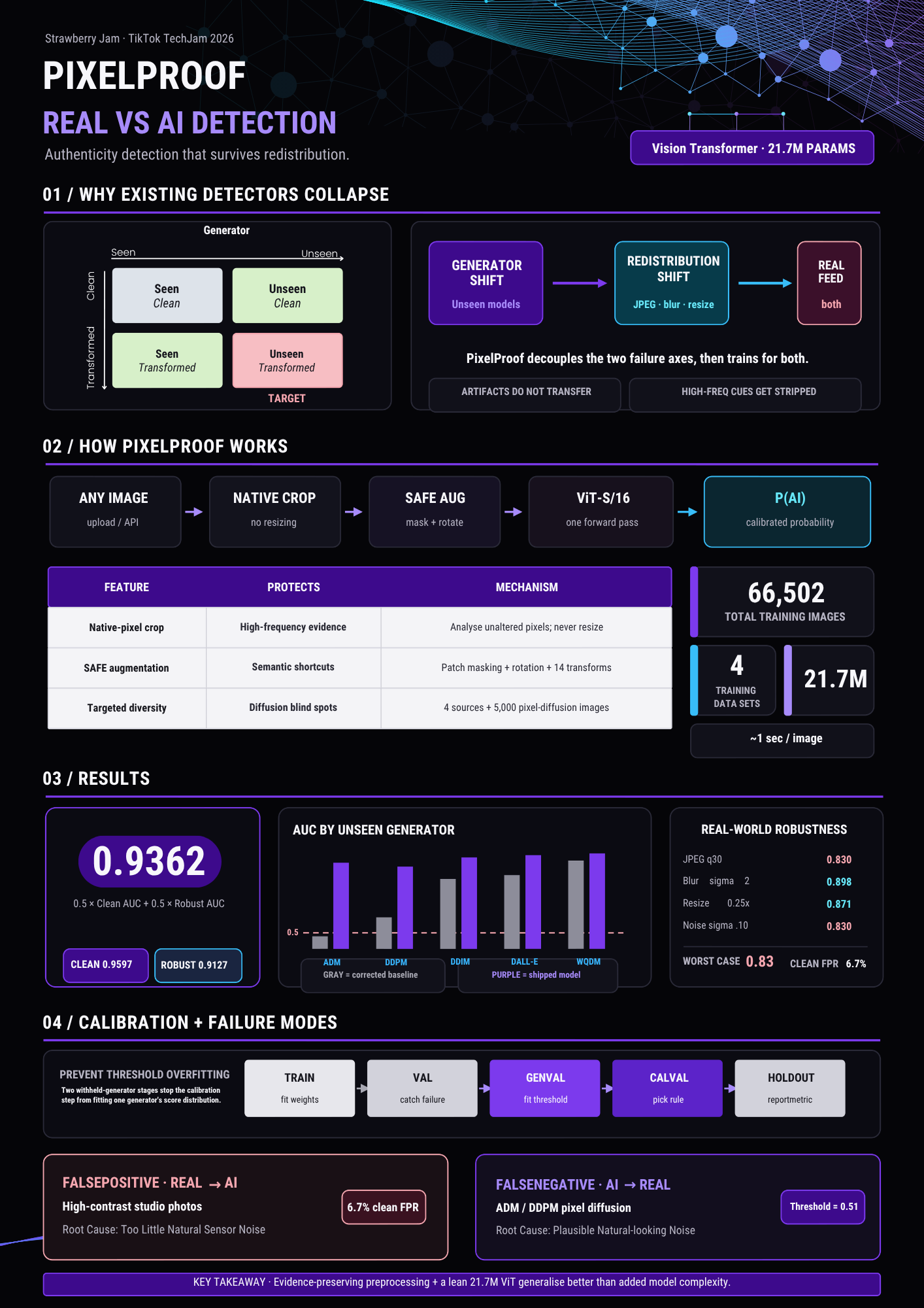
AI-generated images are becoming increasingly difficult to distinguish from authentic photographs. However, real-world images are rarely viewed in their original form. Once uploaded online, they are often compressed, resized, cropped, blurred, or otherwise altered.

Our project addresses a practical question:

Can AI-generated images still be detected reliably after the transformations they experience during online circulation?

We developed a lightweight and robust image detector designed to generalise across previously unseen AI generators, while remaining resilient to common image degradations.

Key Results

MetricResult
Final Score	0.9362
Clean ROC-AUC	0.9597
Robust ROC-AUC	0.9127
Model Size	21.7M parameters
Architecture	ViT-S/16
Ensemble	None
Held-out Generator Families	5

Our final system uses a single Vision Transformer, without additional branches or ensembles.

Inspiration

Many AI-image detectors perform well on clean benchmark datasets, but their performance can deteriorate once images undergo common transformations.

A typical image shared online may experience:

Original Image
      ↓
Social Media Upload
      ↓
JPEG Compression
      ↓
Resize / Crop
      ↓
Blur / Noise
      ↓
Re-upload

These transformations can remove subtle image statistics and high-frequency artifacts that forensic detectors depend on.

We therefore focused on three objectives:

ObjectiveGoal
Generalisation	Detect AI images from generators unseen during training
Robustness	Remain reliable after common image transformations
Efficiency	Keep the model lightweight and practical to run

What It Does

The system receives an image and outputs a probability between 0 and 1, representing the likelihood that it was AI-generated.

              ┌─────────────────────┐
              │     Input Image     │
              └──────────┬──────────┘
                         │
                         ▼
              ┌─────────────────────┐
              │ Native 224×224 Crop │
              └──────────┬──────────┘
                         │
                         ▼
              ┌─────────────────────┐
              │      ViT-S/16       │
              │    21.7M params     │
              └──────────┬──────────┘
                         │
                         ▼
              ┌─────────────────────┐
              │ Classification Head │
              └──────────┬──────────┘
                         │
                         ▼
              ┌─────────────────────┐
              │    P(AI Generated)  │
              │       0 → 1         │
              └─────────────────────┘

For example:

pred = 0.03  → likely authentic
pred = 0.96  → likely AI-generated

The accompanying web application also supports:

Single-image classification
Robustness testing across 15 conditions
Batch image analysis
Confidence scores and CSV export

How We Built It

Our final architecture is intentionally simple:

Image
  ↓
Native-resolution crop
  ↓
ViT-S/16
  ↓
CLS representation
  ↓
Linear classifier
  ↓
AI probability

The most significant improvements did not come from increasing model complexity.

Instead, they came from improving:

preprocessing → training data → evaluation → failure analysis

1. Preserving Native Pixel Evidence

A conventional image pipeline may first resize an image before sending it into a classifier.

Conventional Pipeline

Original Image
      ↓
Resize
      ↓
224×224 Input

Resizing can suppress high-frequency details and alter image statistics that may contain useful forensic evidence.

Our pipeline instead performs a crop directly from the original-resolution image:

Our Pipeline

Original-resolution Image
          ↓
Direct 224×224 Crop
          ↓
ViT

This helps preserve more of the original pixel-level information before inference.

2. Training for Robustness

We also designed the training pipeline to reduce reliance on simple visual shortcuts.

Our augmentation strategy includes:

Random rotation
Patch masking
Native-resolution cropping

The aim is to reduce dependence on factors such as colour distribution, composition, or semantic content and encourage the model to learn more transferable forensic patterns.

3. Designing the Corpus Around Failure Modes

Our final training corpus contains approximately:

66,500 images

from a range of generator architectures.

                  Training Corpus
                        │
        ┌───────────────┼───────────────┐
        │               │               │
        ▼               ▼               ▼
 Latent Diffusion      GANs       Pixel Diffusion
        │               │               │
        └───────────────┼───────────────┘
                        │
                        ▼
                  ViT Training

The training sources include:

DatasetRole
SID_Set	Synthetic-image diversity
DRAGON	Generator diversity
Community Forensics	Multiple architecture families
GenImage ADM / GLIDE	Pixel-space diffusion

This dataset design became one of the most important parts of the project.

A Failure That Changed Our Approach

During early testing, the detector performed poorly on ADM pixel-diffusion images.

Its initial ROC-AUC was:

0.478

This was effectively below chance.

Our training corpus at the time was more heavily represented by other generator architectures, particularly latent-diffusion models.

ADM uses pixel-space diffusion, which produces different forensic characteristics.

We therefore introduced 5,000 ADM/GLIDE images into training.

The result was:

StageADM ROC-AUC
Before targeted data	0.478
After targeted data	0.937

0.478 → 0.937

This was one of the clearest findings of the project:

Improving training-data coverage had a greater impact than increasing architectural complexity.

Robustness Evaluation

The detector was evaluated across the clean condition and 14 required transformations.

TransformationConditions
JPEG Compression	Q90, Q70, Q50, Q30
Gaussian Blur	σ0.5, σ1, σ2
Resize	0.5×, 0.25×
Gaussian Noise	σ0.02, σ0.05, σ0.10
Colour Jitter	±20%
Centre Crop	80%

Selected Results

ConditionROC-AUC
Clean	0.960
JPEG Q90	0.938
JPEG Q50	0.890
JPEG Q30	0.830
Blur σ1	0.955
Resize 0.5×	0.958
Noise σ0.10	0.830
Colour Jitter	0.957
Centre Crop	0.949

The most difficult conditions were:

Heavy JPEG compression
Strong Gaussian noise

Both achieved an ROC-AUC of 0.830.

These transformations directly alter or remove the high-frequency information commonly used by forensic detectors.

Generalisation to Unseen Generators

A key requirement of the project was testing on generator families that were not represented during training.

Organiser Benchmark

GeneratorClean AUCRobust AUC
ADM	0.937	0.870
DDPM	0.913	0.855
DDIM	0.970	0.918
DALL·E	0.984	0.962
VQDM	0.995	0.958

All five generator families were fully held out from training.

This allowed us to evaluate whether the detector had learned transferable forensic patterns rather than simply memorising characteristics of known models.

Overall Performance

BenchmarkFinal ScoreClean AUCRobust AUC
Organiser Benchmark	0.9362	0.9597	0.9127
DRAGON	0.9779	0.9883	0.9675
SID_Set	0.8481	0.8576	0.8386

SID_Set was the most challenging evaluation because it also contains locally manipulated photographs.

Our system performs whole-image classification:

"Was this image generated?"

It is not designed for localisation tasks such as:

"Which region of this photograph was edited?"

What Did Not Work

We experimented with several additional branches to determine whether frequency-domain or semantic features could further improve generalisation.

ApproachHeld-out ResultDecision
DWT Wavelet Branch	No meaningful improvement	Removed
Frozen CLIP-B Branch	No measurable improvement	Removed
FFT Spectrum Branch	0.457 unseen AUC	Removed
Single ViT	0.9362 Final Score	Selected

One of our larger two-branch models contained approximately 108M parameters.

It achieved essentially the same performance as the final 21.7M-parameter model.

108M parameters   ─────────────► 0.9362

21.7M parameters  ─────────────► 0.9362

Given identical performance, we selected the smaller system.

This reduced complexity while improving reproducibility and inference efficiency.

Identifying a Benchmark Shortcut

One of the most important findings during development came from analysing our own evaluation setup.

Our initial organiser-set score was:

0.8131

We then tested a deliberately simple classifier that used only image dimensions.

It achieved:

ROC-AUC = 1.000

This revealed a dataset shortcut.

AI Images
   ↓
Mostly fixed 256×256 resolution

Authentic Images
   ↓
Normal photographic resolutions

A classifier could therefore distinguish the two classes without analysing the actual image content.

We rebuilt the evaluation set with resolution-matched images.

Before Matching
Size-only AUC = 1.000

        ↓

Resolution Matching

        ↓

After Matching
Size-only AUC = 0.500

We then re-evaluated the detector using the corrected dataset.

Although this reduced the reported performance, it produced a substantially more meaningful benchmark.

A benchmark result is only useful if the benchmark itself does not provide unintended shortcuts.

Engineering Trade-Offs

Trade-OffDecision
Clean accuracy vs robustness	Prioritised robustness
Seen vs unseen generators	Prioritised generalisation
Model size vs complexity	Selected smaller model
Higher apparent score vs evaluation validity	Corrected the benchmark
Ensemble vs reproducibility	Used a single model

One particularly important result was:

Seen Validation AUC
0.9866 → 0.9807

Held-out Final Score
0.8804 → 0.9362

Although performance on the seen validation set decreased slightly, performance on unseen generators improved significantly.

For this project, we considered this the more meaningful outcome.

Interactive Demo

The project also includes a web interface with three primary workflows:

                     ┌──────────────┐
                     │     Demo     │
                     └──────┬───────┘
                            │
            ┌───────────────┼───────────────┐
            │               │               │
            ▼               ▼               ▼
       Single Image     Robustness        Batch
                         Testing         Analysis

Single Image

Upload an image and receive a probability and classification.

Robustness Testing

Apply the supported transformations to the same image and compare its predictions across conditions.

Batch Analysis

Evaluate up to 200 images and export the results as a structured table or CSV.

Efficiency

Our final model contains:

21,666,049 parameters

This is approximately 92× below the 2B parameter limit.

Its architecture remains straightforward:

Image
  ↓
ViT
  ↓
Prediction

The final system requires:

One checkpoint
One inference branch
No ensemble
No fusion network
No secondary feature extractor

It can also perform inference on a laptop CPU at approximately one second per image.

What We Learned

Our largest lesson was that improvements in AI-generated image detection do not necessarily come from larger models.

Our most effective development cycle became:

Evaluate
   ↓
Identify Failure
   ↓
Analyse Cause
   ↓
Improve Data / Preprocessing
   ↓
Retrain
   ↓
Evaluate on Unseen Generators

The project shifted our focus away from asking:

“How can we maximise validation accuracy?”

towards:

“What shortcut is the model relying on, and will that behaviour transfer to unseen generators?”

What We Are Proud Of

Our final system combines:

PropertyResult
Final Score	0.9362
Parameters	21.7M
Architecture	Single ViT
Ensemble	None
Unseen Generator Families	5
Robustness Conditions	15

Beyond the final score, we also documented:

False positives and false negatives
Failed architectural experiments
Robustness measurements
Dataset composition
Benchmark corrections
Training configuration
Evaluation methodology

We believe documenting what failed is just as important as documenting what succeeded.

Limitations

AI-generated image detection remains an open challenge.

Our current system is most affected by:

Heavy JPEG Compression

ROC-AUC: 0.830

Strong Gaussian Noise

ROC-AUC: 0.830

Pixel-Space Diffusion

ADM and DDPM remain more difficult than several latent-diffusion families.

Localised AI Editing

The current system performs image-level classification and does not localise AI-generated regions.

Emerging Generator Architectures

Modern flow and DiT architectures such as SD3, Flux and Firefly remain important areas for future evaluation.

What's Next

Based on our experimental results, the next steps would be:

1. Expand pixel-diffusion training data
              ↓
2. Strengthen compression-focused augmentation
              ↓
3. Improve robustness to strong noise
              ↓
4. Add a lightweight borderline second stage
              ↓
5. Revisit test-time augmentation
              ↓
6. Evaluate modern flow and DiT generators

The improvement from: