PINNs and Needles

• 

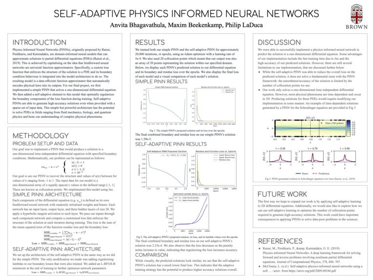
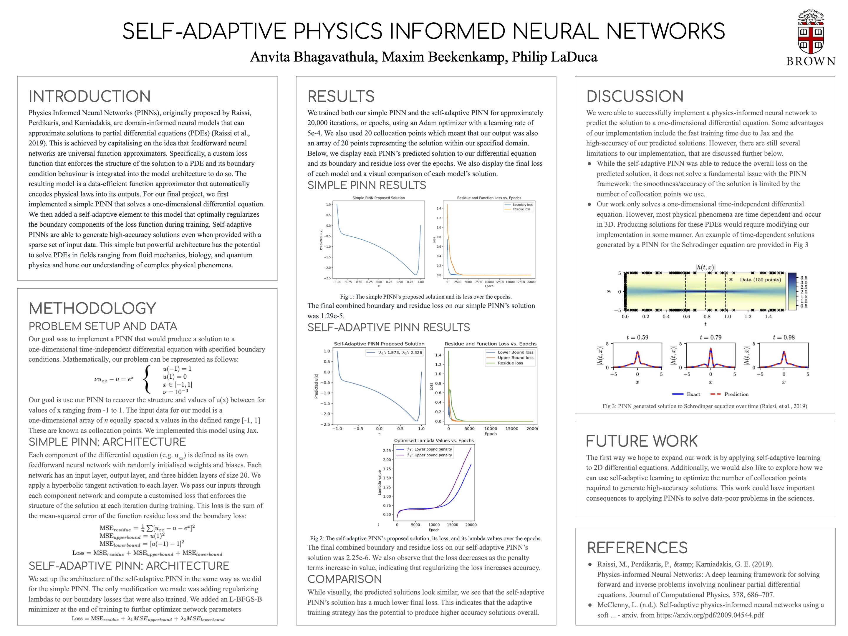
  Final Project Poster

FINAL WRITE-UP/REFLECTION LINK https://docs.google.com/document/d/1zzmesxNs3Yaed0BcaNm9ly9NEX1ZD3L3czyznCyxpHM/edit?usp=sharing

FINAL POSTER (small fixes from the printed version) https://docs.google.com/presentation/d/1NVHiJpvBcL_oaltI7BdUY0BR3deEE5w81De_Ac-riuk/edit#slide=id.p

OUR GITHUB REPO https://github.com/philipladuca24/PINNs-Project

CHECK IN 1

Introduction: We are attempting to re-create a Physics Informed Neural Network, originally proposed in the paper “Physics-informed neural networks: A deep learning framework for solving forward and inverse problems involving nonlinear partial differential equations” by Raissi, Perdikaris, and Karniadakis. Our idea is to create a partial derivative solver that is bound by physical laws, thus improving the accuracy of the solutions. We are motivated by this topic because we are all Physics concentrators and are interested in the intersection between Physics and Deep Learning. We intend to apply the ideas brought by Karniadakis to a physical system they already explore, and then extend the method to different partial derivative systems such as magneto hydrodynamics or thermodynamics. This is a regression problem that involves minimizing/optimizing a loss function to output solutions to differential equations.

Related Work: There are several papers as well as a Github repository form the foundation of the prior work conducted on this topic. They are linked below:

Papers: https://www.sciencedirect.com/science/article/pii/S0021999118307125 https://arxiv.org/abs/1711.10561 https://arxiv.org/abs/1711.10566

GitHub Repo: ​​https://github.com/maziarraissi/PINNs The papers linked above created PINNs for two distinct classes of problems: “data-driven solution and data-driven discovery of partial differential equations”. These problems can likewise be divided into two categories: continuous and discrete time models. The continuous time models look mainly at generically solving PDEs by imposing physical realities onto the network by generic conservation laws. This is because there are possible solutions to partial derivatives which make no physical sense. Short of adjusting the loss functions most of the architectures remain the same between models.The discrete time models look at interpolating data. While building largely on the work established in the continuous portions of the paper, they expand by approaching these problems using Runge-Kutta methods. Runge-Kutta methods are adopted as Bayesian approaches create “robustness/brittleness issues, especially for nonlinear problems” when looking at the arbitrarily large time intervals into the future inherent to the types of problems being solved.

Data: This project involves creating our own datasets using simulations that roughly follow the shape of a given PDE. For instance, in the paper, the researchers simulate data that simulates a PDE using spectral methods and initial states determined by boundary conditions. Training data needs to be randomly sampled from this dataset (the researchers used a Latin hypercube sampling strategy). The researchers have published a number of MATLAB scripts in which they create synthetic data and we hope to recreate one of their examples (in Python) while also extending this analysis to another PDE.

Methodology: The first part of our project involves re-implementing an existing paper (as described above). I believe the hardest part of this project will be data collection and data generation; we will need to familiarize ourselves with the way the researchers have generated synthetic data for each PDE they solved and try to implement this method ourselves. Once we are able to create data for both a PDE that is used in the paper and one of our choice, we will create the PINN neural network and modify the loss functions according to the differential equations. We will then train the neural networks and see how well they are able to fit the data. We will try adding noise to the data set and see how that impacts the results. We will then see how well the neural networks are able to discover the constants in the differential based on data given.

Metrics: Since we will be using PINNs to solve PDEs, we can measure success by looking at how well our model fits the data provided to it. Our base goal is to create and apply a PINN to one of the equations already shown in the paper and achieve similar levels of accuracy. The target goal is to then apply the PINN framework to an equation not already shown in the paper and also achieve an accurate solution. FInally, our stretch goal is to use the PINN to do discovery of differential equations, as shown in the paper, for both an equation given as well as one that is not given.

Ethics: One consideration to make when dealing with neural networks is the energy cost of training the network and collecting and processing the data necessary to get accurate results. One of the main benefits of PINNs is that by constraining the model to only considering physically possible solutions, the neural network is able to more efficiently reach a possible solution which is also, in turn, physically possible. This allows for quicker training times, cutting down on energy cost, as well as smaller datasets required to train accurate models. However, when modifying learning models in this manner, you are explicitly inducing bias into the neural network. That is the whole idea behind constraining the model to physically real solutions to a system. This is contingent on the assumptions being correct which leads to ethical issues regarding how these loss functions are implemented. Instead of models finding solutions solely based on the data provided, they are constrained by human assumption which could lead to biased and malicious results. Another challenge with domain-informed neural networks is with who develops them and who is responsible for their uses; if non domain-experts develop these models and then use them to drive decisions within a given field/industry, this might lead to harmful implications.

Division of Labor: In order to divide the labor each group member will be charged with a different portion of the project. One member will be tasked with producing the datasets for the phenomena we wish to study, another person will be in charge of developing the infrastructure used for the PINN while the final member will focus on applying the PINN to different differential equations.

CHECK IN 2

Introduction: We are attempting to re-create a Physics Informed Neural Network, originally proposed in the paper “Physics-informed neural networks: A deep learning framework for solving forward and inverse problems involving nonlinear partial differential equations” by Raissi, Perdikaris, and Karniadakis. Our idea is to create a partial derivative solver that is bound by physical laws, thus improving the accuracy of the solutions. We are motivated by this topic because we are all Physics concentrators and are interested in the intersection between Physics and Deep Learning. We intend to apply the ideas brought by Karniadakis to a one-dimensional differential equation and generate a solution by training a feed-forward neural network that approximates the solution function. Our idea is to minimize a customized loss function which is a sum of the residual loss of the structure of the solution as well as its expected boundary condition behavior. Extending upon this idea, we also hope to explore solution generation in a data-poor / no-data regime using self-adaptive learning.

Challenges: The most challenging part of this project has been familiarizing ourselves with how Jax works. While there were a number of analogous operations to Tensorflow, we had to learn how functions such as vmap and grad worked to make our code work. Additionally, since our project is very math-heavy, we had to quickly grasp how to translate complex mathematical ideas into Jax. For example, we had to learn how to enforce boundary conditions using a customized loss function. We also needed to learn how to define a number of functions in Jax that represented the various derivatives in the equation we were solving.

Insights: Our model was able to successfully identify the solution to the proposed differential equation, which we evaluated by comparing our solution to the one generated by Wolfram Alpha’s numerical PDE solver. We noticed that our generated graph was quite smooth and accurate when we were using 200 collocation points. However, when we decreased this value to ~20 collocation points, the graph became a lot more jagged and inaccurate. Since a lot of the applications of our work are data-poor, we had to figure out how to overcome this scenario. One idea to do so was to change the weighting of our two custom loss-functions and place less weightage on the boundary loss to enforce the structure of the solution more strongly.

Plan: We are definitely on track with our project. Our current code generates a numerically accurate solution to the one-dimensional differential equation we were examining with a large number of x-value data (collocation points). Our next steps, however, are to focus on generating optimal solutions when we have a limited amount of input collocation points. To tackle this problem, we will try to implement self-adaptive learning in the weightage of our loss functions. In simpler words, we will assign multiplicative parameters lambda_1 and lambda_2 to weight the importance of the function loss and the boundary loss, and try to train these parameters too. Our next steps will be to implement this idea into our code and generate a number of graphs for various values of lambda and observe how our model determines the optimal solution.

Built With

• jax