PhysioTransit

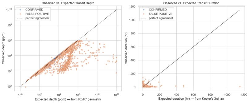
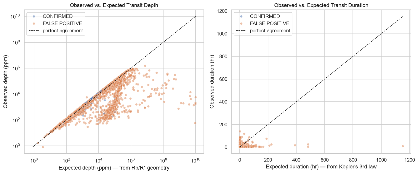
Observed vs Expected Transit Depth and Duration
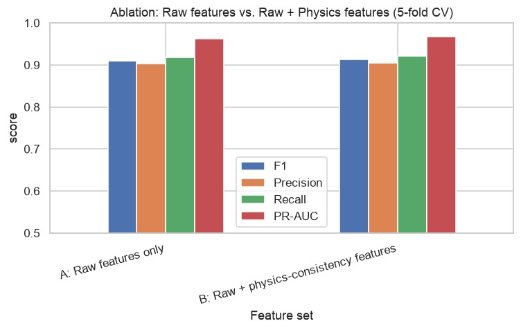
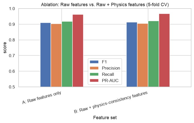
Ablation
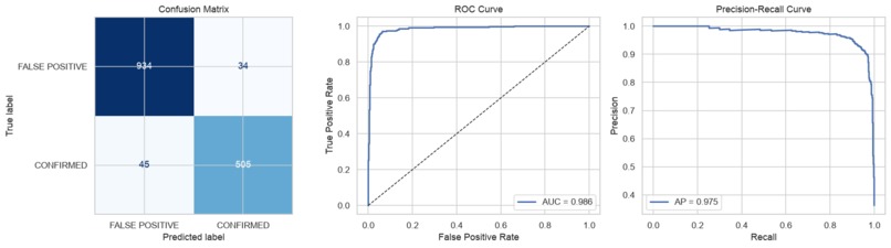
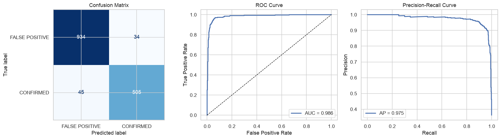
Confusion Matrix + ROC + Precision-Recall Curve
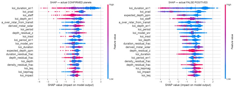
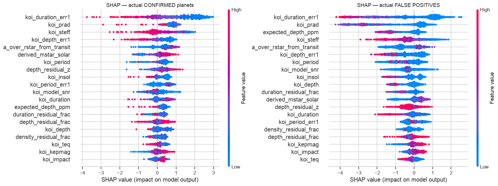
SHAP

Inspiration

The Kepler mission alone flagged over 9,000 signals that looked like they could be planets, and only a fraction turned out to be real. NASA's own vetting pipeline separates confirmed planets from false positives, but most machine learning approaches to this problem just throw raw catalog columns at a classifier and let it find whatever correlations it can. We wanted to try something closer to how an astronomer actually reasons about a candidate: a transiting planet's orbital period, transit duration, transit depth, and host star properties aren't independent numbers, they're linked by orbital mechanics. If a signal is really a planet, those numbers have to agree with each other. If it's an eclipsing binary or a blended background star, the pipeline still fits a "planet" model to it, but the fit won't hold together physically.

What it does

The model takes raw KOI catalog features and adds a set of physics-consistency features on top: for each candidate, we predict what the transit duration and depth should be from Kepler's third law and basic transit geometry, then compute how far the observed values are from that prediction. We also invert the problem and derive a transit-only stellar density directly from the light curve, independent of the catalog's own stellar model, and compare the two. Real planets cluster near agreement on both checks. False positives don't. We feed both the raw features and these physics features into a gradient-boosted classifier, and run an ablation study to see whether the physics features are actually pulling their weight or just adding noise.

How we built it

We started with the standard NASA Exoplanet Archive KOI cumulative table (Celesta's cleaned starter CSV, ~7,600 resolved KOIs after setting aside unresolved CANDIDATE rows). Early development ran on a synthetic dataset we generated ourselves, built to mimic the real table's structure and roughly the physical separation we expected between confirmed planets and false positives, so we could validate the full pipeline end to end before the real data was available. Once the real CSV was in hand, we swapped it in and reran everything.

The pipeline itself: exclude known leakage columns (koi_score, the koi_fpflag_* pipeline judgments), engineer the physics-consistency features, run a stratified train/test split, then compare Logistic Regression, Random Forest, and XGBoost with 5-fold cross-validation. We ran a controlled ablation, same model, same folds, same hyperparameters, comparing raw features alone against raw plus physics features, so any performance difference could only be attributed to the added features. XGBoost came out ahead, and we tuned it with a randomized search, picked a decision threshold off the precision-recall curve instead of using the default 0.5, and only touched the held-out test set once, at the very end.

For explainability we computed SHAP values separately for actual confirmed planets and actual false positives, since what convinces the model something is real isn't necessarily the same as what convinces it something is fake. We cross-checked those SHAP rankings against permutation importance computed directly on the test set, and built a plain-language generator that turns a prediction into a sentence a non-technical reader can follow.

Results

On the held-out test set, the final model reached an F1 of 0.9275 and ROC-AUC of 0.986. The ablation showed the physics features improved every metric over raw features alone, F1 went from 0.910 to 0.913, ROC-AUC from 0.979 to 0.982. The gain is real but modest, which told us the raw catalog features were already carrying a lot of the signal on their own. Where the physics features mattered most was specifically in flagging false positives: one of them, the expected transit depth from Rp/R* geometry, ranked as the third most important feature by SHAP for false positive predictions, but only thirteenth for confirmed planets.

Challenges we faced

Getting the physics derivations right was the hardest part. Small errors compound: an error in the semi-major axis calculation throws off the expected duration, which throws off the residual, which quietly poisons the feature the whole project depends on. We had to be explicit about every assumption (circular orbits, near-edge-on inclination, stellar mass derived from surface gravity since it isn't given directly in the catalog) rather than letting them hide inside the math.

Handling missing data honestly was another one. Several columns, particularly the per-value uncertainty columns, have a meaningful chunk of missing values in the real table. We chose to let missingness propagate as NaN through feature engineering and only impute inside the modeling pipeline, so we never accidentally fabricated a "physically consistent" result out of missing inputs.

Error analysis surfaced a pattern we didn't expect going in: the model's remaining false negatives, the real planets it misses, cluster around low signal-to-noise candidates rather than around any particular physics residual. Its false positives, the ones it wrongly flags as real, tend to have longer orbital periods and smaller residuals than typical false positives, meaning they're genuinely borderline cases rather than outright violations of the physics.

What we learned

Domain knowledge doesn't replace a good model, but it does change what the model can see. The most useful lesson was in how we validated the ablation itself: it would have been easy to just report that the physics-augmented model scored higher and call it a day, but holding the algorithm, folds, and hyperparameters fixed across both runs is what makes that comparison mean anything at all.