-

ThumbNail
-
F1_Score Analysis
-
Cohen_Kappa Score

Dataset Challenge Description
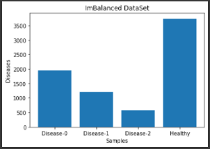
The bacteria in the gut microbiomes of persons with various disorders make up the dataset. There are 1949 disease-0 samples, 1213 disease-1 samples, 578 disease-2 samples, and 3741 healthy samples. Each row represents a sample taken from a single person, whereas each column represents a bacteria found in at least one person's gut microbiome. Each sample's label is listed in the "disease" column.

Challenges
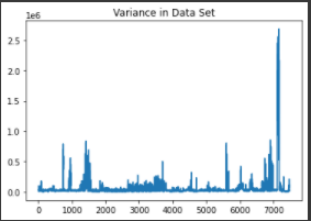
High Variance in Sum of Microorganisms
In order to combat this problem, we standardized the microorganisms in order to have similar value ranges (feature scaling). The idea is to bring down all the features to a common scale without changing the differences in the range of the values. Feature scaling is useful in making gradient descent converge faster. By ensuring that the sum of all the microorganisms in each sample is standardized, we get more consistent data points and as a result, we can expect better model performance.
Imbalanced DataSet
Our initial approach to deal with the unbalanced data was to oversample the minority classes by duplicating random samples within the class. We ensured the same amount of samples in each classification for the training data to impersonate a balanced dataset. Unfortunately, this did not achieve a high f1 score due to the fact that a class had a much smaller sample size and hence we had to duplicate it three times over which caused overfitting.
We accounted for the unbalanced dataset by implementing SMOTE Techniques. SMOTE allows us to create synthetic samples for the minority classes ( the diseases) by estimating samples in specific regions. SMOTE basically allowed us to go from an imbalance dataset of 7840 samples to a balanced dataset of over 14000 where each label had the same amount of samples of 3741.
Iteration of Algorithms
KNN
In order to optimize the accuracy of our ML model, we needed to test multiple algorithms to see which yielded a greater accuracy. We tested the K nearest neighbors algorithm to determine if it was accurate. To use knn effectively it is important to preprocess the data on an n-dimensional graph. We then place the incoming data in the graph and check K neighbors to see which classification it belongs in. In this case we came to the conclusion that 20 neighbors was optimal for this algorithm. Unfortunately, this algorithm only yielded a 0.70 f1 score.
| Score | Mean |
|---|---|
| F1 Score | 0.70 |
Naive bayes
We then experimented with naive Bayes. This algorithm is mostly suited for categorical classification, however there are some variations that can handle numerical data. Gaussian naive Bayes was ruled out because it uses mean and variance so knowing our data has substantial variety in feature sums, we ruled this one out. Complement naive Bayes was the next best choice as it takes into account imbalance datasets in its probability calculation. Unfortunately, it only produced an f1 score of 0.59 and Cohen kappa score of 0.39 even with laplace smoothing that takes into account zero value features.
| Score | Mean |
|---|---|
| F1 Score | 0.71 |
| Cohen-Kapp | 0.39 |
SVM
We also used the SVM algorithm, a ML model that utilizes an n dimensional graph where we plot preprocessed data based on their features. The svm algorithm plots a hyperplane that separates different clusters of points with different classifications. Based on incoming data, the algorithm classifies it based on its position relative to the hyperplane. This algorithm yielded a 0.65 f1 score.
| Score | Mean |
|---|---|
| F1 Score | 0.65 |
Decision tree
This algorithm is well suited for data with outliers but they generally perform poorly in comparison to other models because of overfitting. For our experimentation, we did hyperparameter tuning to choose the best model. First, we tested for the max_depth value which was 14. Then, we found that between the gini index and entropy, entropy is the better criterion to use for the algorithm. These criteria allow us to calculate the impurity of a node and adjust the decision tree accordingly. We also tested for the best random state value which was found to be 183. After choosing a model with these best suited hyperparameters, this model gave us an f1 score of 0.71 and a Cohen kappa score of only 0.55.
| Score | Mean |
|---|---|
| F1 Score | 0.71 |
| Cohen-Kapp | 0.55 |
Our Final Algorithm to the Problem : Recurrent Neural Network(RNNs) with SMOTE technique for dealing with Imbalance Data
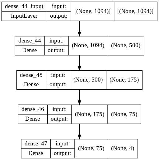
For our final submission, we have decided to create a simple sequential rectified model with an output layer of activation of soft-max in order to see the probability of each label. Our neural network contains 4 hidden layers and compresses the initial 1094 bacteria into 500 neurons, then 175 neurons, then 75 neurons and finally 4 which corresponds to the number of labels required. The resulting neurons will each have a probability of its being the accurate class. We choose the class with the highest probability to be the classification.
Final Results
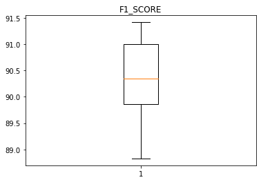
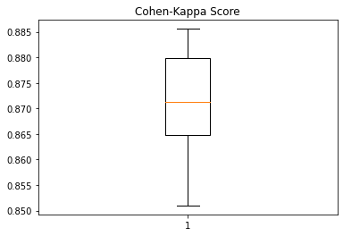
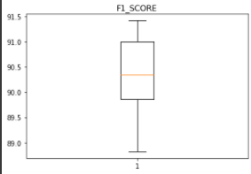
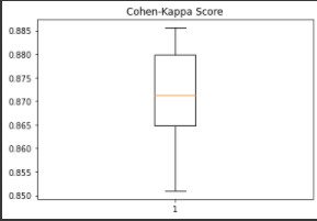
In order to test our model, we used cross-validation over 10 iterations to determine the mean of F1_Score and Cohen-Kapp.
| Score | Mean |
|---|---|
| F1 Score | 0.905 |
| Cohen-Kapp | 0.875 |
Built With
- anaconda
- jupyter
- keras
- matplotlib
- python
- tensorflow


Log in or sign up for Devpost to join the conversation.