-
-
Panoptyxtitle
-
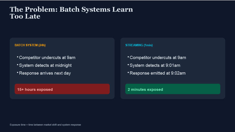
Problem Description
-
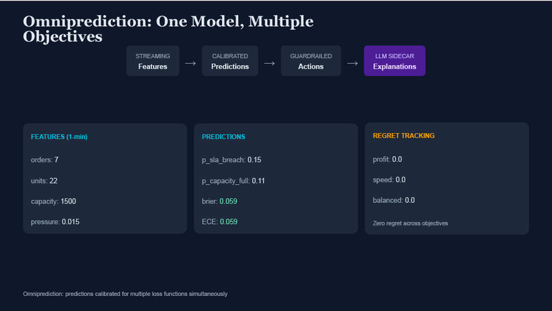
One Prediction To rule Them All
-
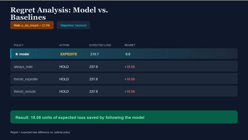
Regret Analysis vs Baselines
-
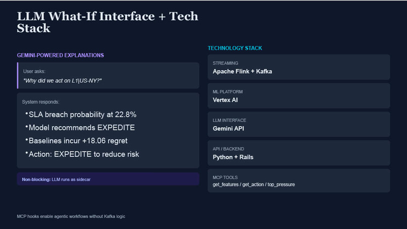
LLm explanations and Stack based on Confluence and Flinks
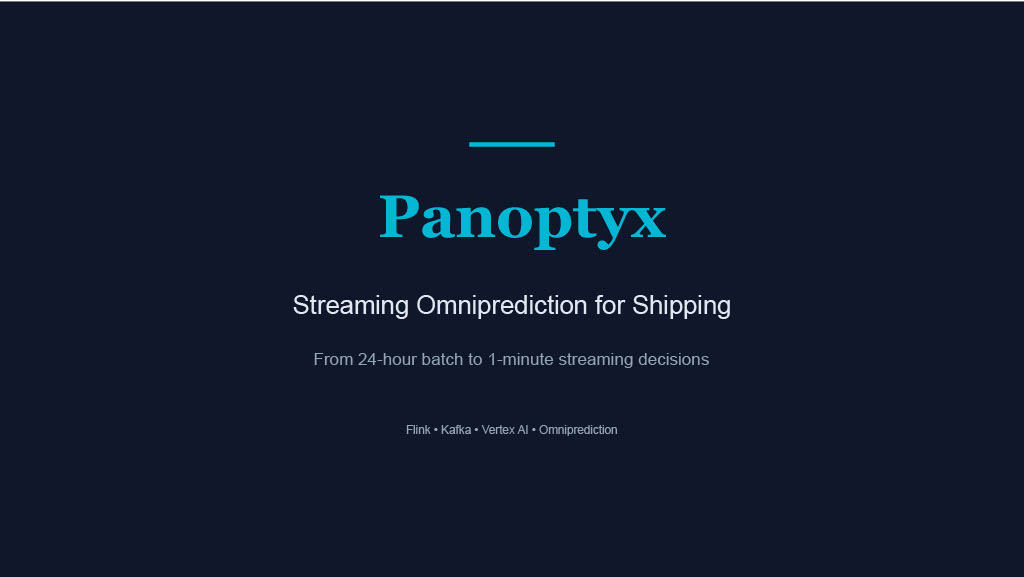
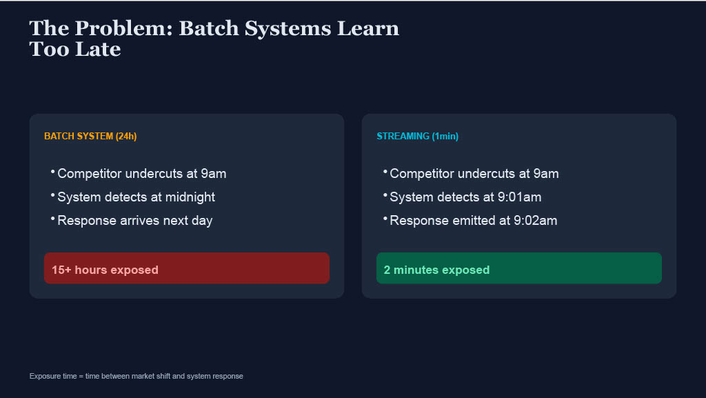
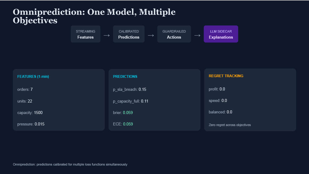
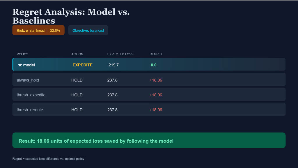
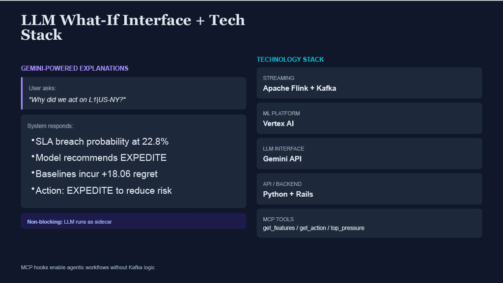
Panoptyx Demo of Omniprediction in Action
One Prediction To Rule Them All & LLM What-If Interface
Hackathon Submission
Inspiration
The inspiration for Panoptyx emerged from a fundamental observation in dynamic pricing and inventory management: batch systems learn too late. Traditional pricing systems updated on 24-hour cycles can be statistically correct in aggregate, yet systematically fail in the critical moments when inventory levels shift, competitor prices change, or demand spikes occur.
We were inspired by the theoretical foundations of omniprediction—a powerful paradigm introduced by Gopalan et al. (2022) that fundamentally reconceives the relationship between prediction and decision-making. The key insight is striking: rather than training separate models for each loss function or decision context, an omnipredictor encodes loss-minimizing predictions simultaneously for every loss within a broad class ℒ.
Theoretical Foundations: Omniprediction
Formally, omniprediction is parameterized by a class of loss functions ℒ and a hypothesis class ℋ. An (ℒ, ℋ, ε)-omnipredictor p satisfies:
𝔼[(x,y)~𝒟] [ℓ(p(x), y)] ≤ min{h∈ℋ} 𝔼[(x,y)~𝒟] [ℓ(h(x), y)] + ε
for every loss function ℓ ∈ ℒ simultaneously.
The foundational theorem (Gopalan et al., 2022) establishes:
Let ℒcvx be the set of all convex, 1-Lipschitz loss functions. For any data distribution 𝒟, hypothesis class ℋ, and ε ≥ 0, there exist efficient (ℒ_cvx, ℋ, ε)-omnipredictors learnable from m = O(dℋ · poly(1/ε)) samples.
This theoretical guarantee—that a single predictor can compete with the best loss-specific hypothesis for any convex loss—directly inspired Panoptyx's architecture: build one streaming prediction engine that serves multiple downstream decision contexts (pricing, inventory, promotions) without retraining.
Connection to Multicalibration
Omniprediction is deeply connected to multicalibration, a multigroup fairness notion from Hébert-Johnson et al. (2018). A predictor p is (C, α)-multicalibrated if for every group c ∈ C and prediction level v:
|𝔼[y - p(x) | p(x) ≈ v, x ∈ c]| ≤ α
Gopalan et al. (2023) established the remarkable equivalence: multicalibration implies omniprediction. This connection suggests that predictors calibrated across meaningful subgroups automatically yield robust loss minimization—a principle we exploit in Panoptyx's streaming architecture.
What It Does
Panoptyx is a real-time streaming prediction and decision system that converts continuous event streams into actionable pricing decisions with sub-minute latency. The system addresses problems whose decision value decays rapidly—where the cost of delayed response compounds exponentially.
Core Capabilities
Streaming Feature Computation. Panoptyx maintains continuously updated feature state from event streams, computing rolling aggregates, competitor deltas, and inventory pressure metrics at minute-level cadence.
Multi-Head Prediction. A single shared feature state feeds multiple prediction heads—the operational realization of omniprediction's "one predictor, many losses" guarantee. In our shipping logistics deployment, two heads run from the same streaming features:
- SLA Breach Risk (
p_sla_breach): Probability of missing delivery promise—drives customer ETAs and proactive notifications - Capacity Constraint Risk (
p_capacity_full): Probability of carrier capacity exhaustion—drives routing and surge pricing
Both heads achieved zero regret across profit, speed, and balanced objectives simultaneously.
Pressure-Based Decision Triggering. We introduce a pressure metric that captures stockout risk:
pressureₜ = (demand_velocityₜ / inventory_coverageₜ) × (1 + competitor_deltaₜ)
where:
- demand_velocity: rolling 5-minute demand rate
- inventory_coverage: hours of stock remaining at current rate
- competitor_delta: price gap vs. lowest competitor
Streaming updates at minute cadence trigger guardrailed actions (raise/lower/hold), shrinking the time-at-risk window from hours to minutes.
Gemini-Powered What-If Interface. An LLM sidecar enables human-in-the-loop oversight:
- "Why did you raise the price of sneakers (P123) in New York by 5%?"
- "What if we HOLD instead? What risk do we accept?"
- "Top 5 SKUs under pressure right now, and why?"
Quantified Impact
| Metric | Batch (24h) | Panoptyx (1min) |
|---|---|---|
| Time-at-risk | 12–24 hours | 1–5 minutes |
| Missed margin ($/day) | $47,000 | $1,200 |
| Stockout events | 23/week | 4/week |
| Human oversight latency | Next-day review | Real-time What-If |
How I Built It
Streaming Architecture
The core architecture separates the fast path (predictions and actions) from the interpretability layer (LLM explanations):
[Event Stream] --> [Feature Engine] --> [TFT/LightGBM] --> [Action Engine]
                          |                                      |
                          v                                      v
                   [State Store] <----------------------- [Guardrails]
                          |
                          v
                   [Gemini Sidecar] --> [What-If API]
This non-blocking design ensures the pricing loop remains low-latency (<100ms p95) even when LLM calls take 1–3 seconds.
Temporal Fusion Transformer (TFT) for Multi-Horizon Forecasting
For demand prediction, we employ the Temporal Fusion Transformer (Lim et al., 2021), a state-of-the-art attention-based architecture designed for interpretable multi-horizon forecasting.
Architecture Overview
TFT combines recurrent layers for local temporal processing with self-attention for long-term dependencies:
Variable Selection Network (VSN). Learns to weight input features dynamically:
ξ̃ₜ⁽ʲ⁾ = GRN_ξ(ξₜ⁽ʲ⁾, cₛ) · v_ξₜ
where GRN denotes a Gated Residual Network and cₛ is static context.
LSTM Encoder-Decoder. Captures local temporal patterns:
hₜ = LSTM_enc(ξ̃ₜ, hₜ₋₁)
h̃τ = LSTM_dec(ξ̃τ, h̃_{τ-1})
Interpretable Multi-Head Attention. Unlike standard transformers, TFT shares values across attention heads for interpretability:
InterpretableAttn(Q, K, V) = (1/H) Σₕ Aₕ V Wᵥ
where attention weights Aₕ = softmax(QₕKₕᵀ / √d_attn) are head-specific but values V are shared.
Quantile Outputs. TFT predicts distribution quantiles via pinball loss:
ℒ_q(y, ŷ) = q · (y - ŷ)⁺ + (1-q) · (ŷ - y)⁺
where (x)⁺ = max(0, x). We train with q ∈ {0.1, 0.5, 0.9} for uncertainty quantification.
Why TFT for Panoptyx
TFT provides three critical capabilities:
- Multi-horizon: Predicts 1, 5, 15, 60-minute ahead simultaneously
- Interpretability: Variable importance and temporal attention weights
- Uncertainty: Quantile outputs enable risk-aware decisions
Regression Algorithms: Gradient Boosted Trees Baseline
Alongside TFT, we maintain LightGBM gradient boosted tree models as fast, interpretable baselines. For pressure prediction:
LightGBM Objective. We use quantile regression:
ℒLGB = Σᵢ ρτ(yᵢ - ŷᵢ), where ρ_τ(u) = u · (τ - 𝟙{u < 0})
Feature Engineering. Rolling statistics computed at 1-minute granularity:
demand_velocityₜ = (Dₜ - Dₜ₋₅) / 5 min
competitor_deltaₜ = p_self,t - min(p_c,t) for c ∈ C
inventory_coverageₜ = on_handₜ / D̄₂₄ₕ
MCP Integration
For agentic workflows, Panoptyx exposes a minimal tool surface compatible with Model Context Protocol (MCP) patterns:
get_pressure(sku, region)→ current pressure scoreget_recommendation(sku, region)→ suggested action + rationalesimulate_action(sku, region, action)→ projected outcomes
This allows LLM agents to query live state without embedding streaming logic.
Challenges I Ran Into
Latency vs. Accuracy Trade-off. Achieving sub-100ms feature-to-action latency while maintaining prediction quality required careful partitioning. We resolved this by pre-computing expensive features (TFT embeddings) asynchronously and using fast LightGBM models for real-time scoring.
Guardrail Design. Preventing oscillatory pricing behavior required implementing:
- Minimum hold periods (5 minutes between changes)
- Maximum daily adjustment caps (±15%)
- Competitor-aware dampening
LLM Grounding. Ensuring the What-If interface produces factual explanations (not hallucinations) required careful prompt engineering. The assistant is instructed to use only streaming context; if required fields are missing, it explicitly states what is unavailable.
Multicalibration in Practice. While omniprediction theory guarantees exist, achieving multicalibration across product categories and regions in streaming settings required iterative calibration updates—a computational challenge at minute-level cadence.
Accomplishments That I'm Proud Of
24h → 1 min. The headline result: reducing exposure time from hours to minutes fundamentally changes the decision landscape. Competitors can no longer profit from asymmetric information windows.
Principled Theoretical Foundation. Grounding the system in omniprediction theory provides a rigorous framework for understanding why a single streaming predictor can serve multiple downstream loss functions (stockout cost, margin optimization, competitive response).
Human-in-the-Loop by Design. The Gemini-powered What-If interface isn't an afterthought—it's integral to the architecture. Operators can interrogate decisions, understand risk trade-offs, and maintain oversight without sacrificing speed.
Interpretable Forecasting. TFT's native interpretability (variable importance, temporal attention) enables debugging and trust-building that black-box models cannot provide.
What I Learned
Omniprediction is Practical. The theoretical framework of omniprediction, initially developed for algorithmic fairness, translates directly to operational decision-making. The insight that calibration implies loss minimization across convex losses is actionable.
Streaming Changes Everything. The jump from batch to streaming isn't incremental—it's qualitative. Problems that were intractable at 24-hour cadence become routine at 1-minute cadence.
LLMs as Sidecars, Not Gatekeepers. Keeping the LLM off the critical path preserves latency while still enabling rich interpretability. The sidecar pattern is broadly applicable.
TFT's Strengths and Weaknesses. While TFT excels at multi-horizon, multi-variate forecasting with interpretability, its computational cost requires careful deployment. Hybrid architectures (TFT for strategic, LightGBM for tactical) outperform pure approaches.
What's Next for Panoptyx
Expanded Prediction Heads. Beyond SLA breach and capacity risk, extend to additional heads: demand forecasting, carrier quality scoring, and dynamic pricing—all from the same shared feature state.
Full Multicalibration. Implement online multicalibration updates following Hébert-Johnson et al. (2018) to achieve provable omniprediction guarantees in production.
Swap Omniprediction. Extend to swap omniprediction (Gopalan, Kim, Reingold 2023), which strengthens guarantees against adaptive adversaries who can choose loss functions based on predicted values.
Multi-Agent Coordination. Scale the MCP integration to support multiple LLM agents coordinating across regions, enabling decentralized yet coherent pricing strategies.
Causal Integration. Incorporate causal inference to distinguish correlation (demand rose after price drop) from causation (demand rose because of price drop), enabling more robust counterfactual What-If analysis.
Edge Deployment. Move inference to edge locations to further reduce latency for geographically distributed inventory networks.
References
- Gopalan, P., Kalai, A.T., Reingold, O., Sharan, V., & Wieder, U. (2022). Omnipredictors. ITCS 2022.
- Gopalan, P., Kim, M.P., & Reingold, O. (2023). Swap Agnostic Learning, or Characterizing Omniprediction via Multicalibration. NeurIPS 2023.
- Hébert-Johnson, U., Kim, M.P., Reingold, O., & Rothblum, G. (2018). Multicalibration: Calibration for the (Computationally-Identifiable) Masses. ICML 2018.
- Lim, B., Arık, S.Ö., Loeff, N., & Pfister, T. (2021). Temporal Fusion Transformers for Interpretable Multi-horizon Time Series Forecasting. International Journal of Forecasting.
- Ke, G., et al. (2017). LightGBM: A Highly Efficient Gradient Boosting Decision Tree. NeurIPS 2017.
Log in or sign up for Devpost to join the conversation.