-
-
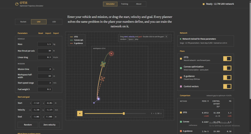
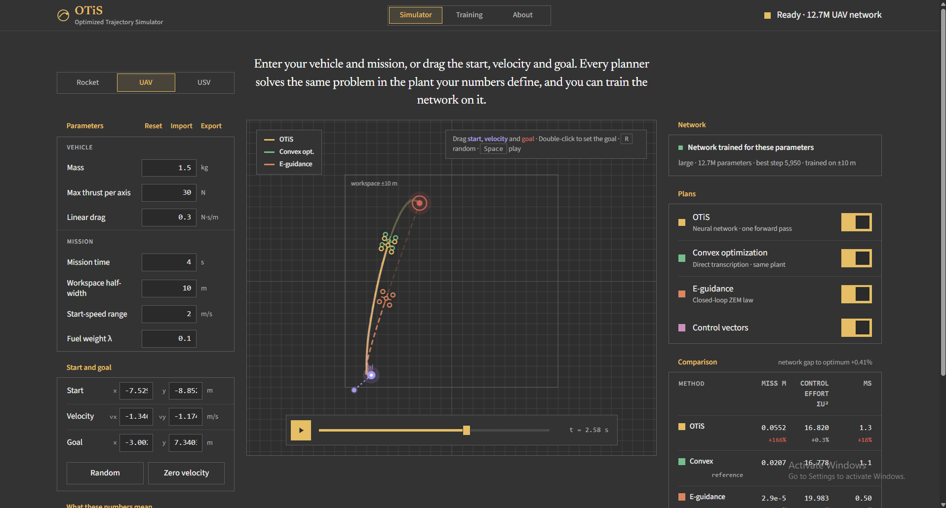
Simulator Page
-
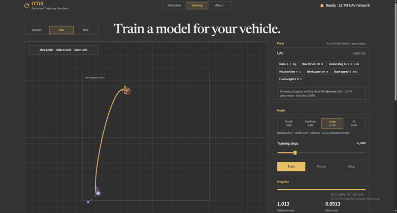
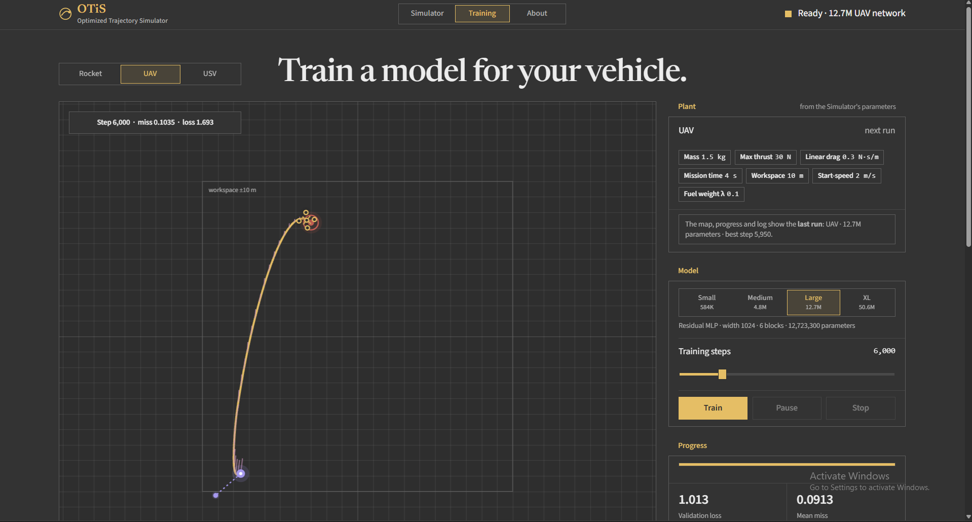
Training Page
-
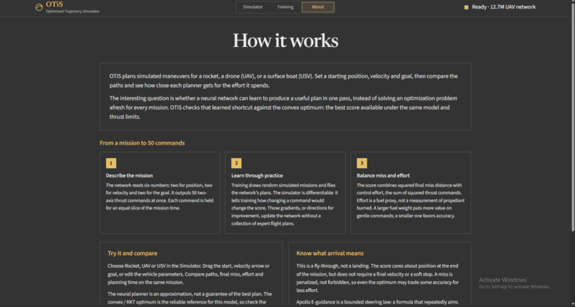
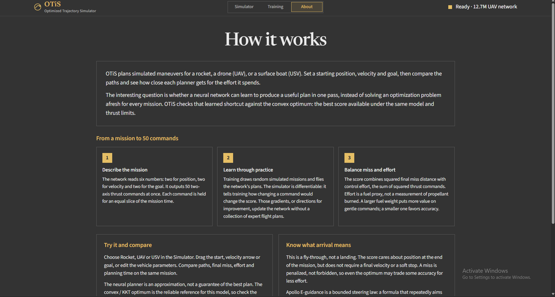
About Page
-
Logo
Inspiration
Ahan conducts robotics research and Madhav has a background in AI/ML research, and in both worlds we kept running into the same wall. The tools for planning how robots and spacecraft move are powerful, but they sit behind expensive compute, specialized solvers and years of control-theory background. Flight systems like JPL's G-FOLD and SpaceX's Falcon 9 landing guidance solve a fresh optimization problem for every maneuver, and learning-based alternatives usually need huge datasets of expert solutions or long reinforcement-learning runs.
We think that technology shouldn't be limited to teams with large budgets and compute clusters. What if a student with one consumer GPU could train a near-optimal planner for their own vehicle in minutes, using nothing but its physics? That question became OTiS: a neural network that learns by backpropagating through a differentiable physics simulator, with no dataset, no labels and no reinforcement learning. It trains in under three minutes on a single GPU, plans a mission in about a millisecond, and lands within 0.018% of the mathematically provable optimum.
What it does
Give OTiS a vehicle's start position, velocity and a target, and a neural network writes the entire plan (50 thrust commands over 4 seconds) in one forward pass. The interactive simulator flies that plan next to the industry baselines, so you can drag a goal and compare miss, fuel and solve time live. You can also define your own vehicle (mass, thrust, drag, mission time, fuel weight) and train a network for its physics with one click.
How we built it
A training loop with no dataset. Every training step:
- Generate 1,024 random missions (start, velocity, goal).
- The network, a 12.7 M-parameter residual MLP in Flax, writes 50 thrust commands per mission.
- Fly them through a physics simulator written in JAX (
lax.scan), so the entire rollout is differentiable. - Score each plan on miss and fuel:
$$J = \lVert p_N - g \rVert^2 + \lambda \sum_{k=0}^{49} \lVert u_k \rVert^2, \qquad |u_k| \le 1,\ \lambda = 0.01$$
Baselines, all flown through the same simulator and scored with the same J:
- Convex optimization (CVXPY + Clarabel), the flight-proven status quo, with OSQP as an independent cross-check.
- Apollo E-guidance, the closed-form law
a = 3·ZEM / t_go².
Results on 5,000 missions the network never saw (5 folds × 1,000):
| Metric | Result |
|---|---|
| Mean gap to the exact optimum | 0.0184% (95% CI 0.0145–0.0238%) |
| Median / p99 gap | 0.0016% / 0.323% |
| vs convex solver | Ties it on the objective |
| vs Apollo E-guidance | Better on 99.4% of missions |
| Batched throughput | 117× the convex solver |
The front end is plain HTML, CSS and JavaScript served by Python, with training and benchmarks run from the command line on the GPU under WSL2.
Challenges we faced
- Building a fair comparison. It's easy to make a neural network look good. We flew every method through one simulator, scored them with one objective, computed the true optimum, and drew test missions from random streams the trainer never touches.
- Stiff problems. High thrust-to-weight with a small fuel weight barely trains: a UAV at λ = 0.01 was still 495% from optimal after 3,000 steps, versus 4.2% at λ = 0.1. We traced it to the condition number κ = 1 + ‖b‖²/λ and added a live κ readout that warns before you train.
- Out-of-distribution behavior. With starting velocities 2× wider than training, the gap rises to 1.99%. Because our training data is generated, the fix is simply to widen the sampling range.
What we learned
- Physics can be the dataset. A differentiable simulator gives an exact training signal, which is why training takes minutes rather than the long runs reinforcement learning needs.
- Math predicts learnability. One number, the problem's condition number, told us in advance which vehicles would train quickly and which would struggle.
- Verification is half the work. We cross-checked every layer: the simulator against the closed-form solution and SciPy's DOP853 (to 10⁻⁶), the gradients against finite differences, and two independent solvers against the exact optimum (to 10⁻⁸).
What's next for OTiS
- Nonlinear dynamics (6-DOF, aerodynamics, orbits), where no closed-form optimum exists.
- Using the network's plan to warm-start a convex solver, combining neural speed with solver guarantees.
Built With
- clarabel
- css3
- cuda
- cvxpy
- differentiable-programming
- flax
- html5
- javascript
- jax
- machine-learning
- matplotlib
- numpy
- nvidia
- optax
- optimal-control
- osqp
- python
- scipy
- wsl2

