-
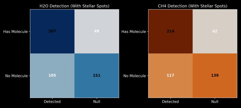
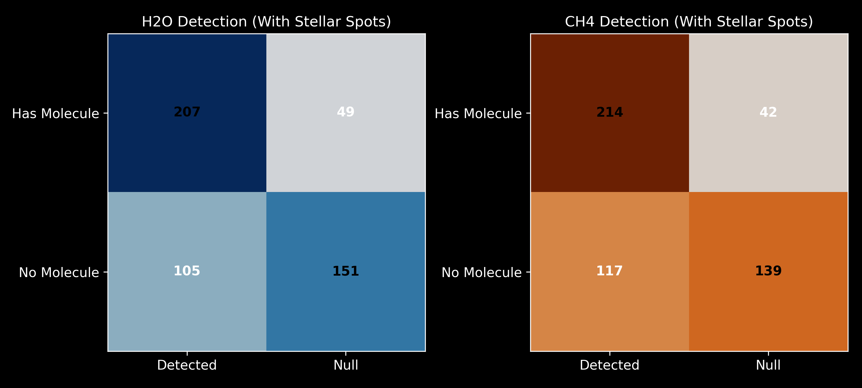
confusion matrix
-
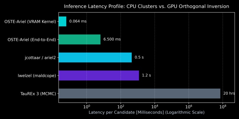
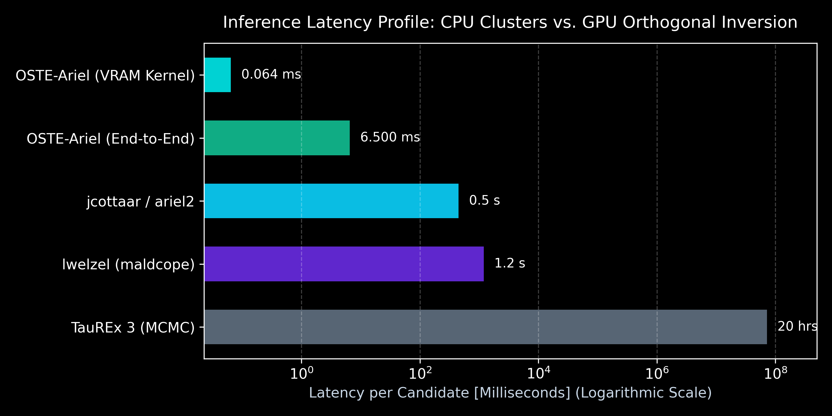
latency breakdown
-
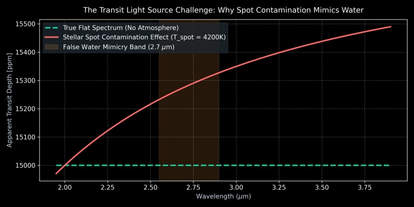
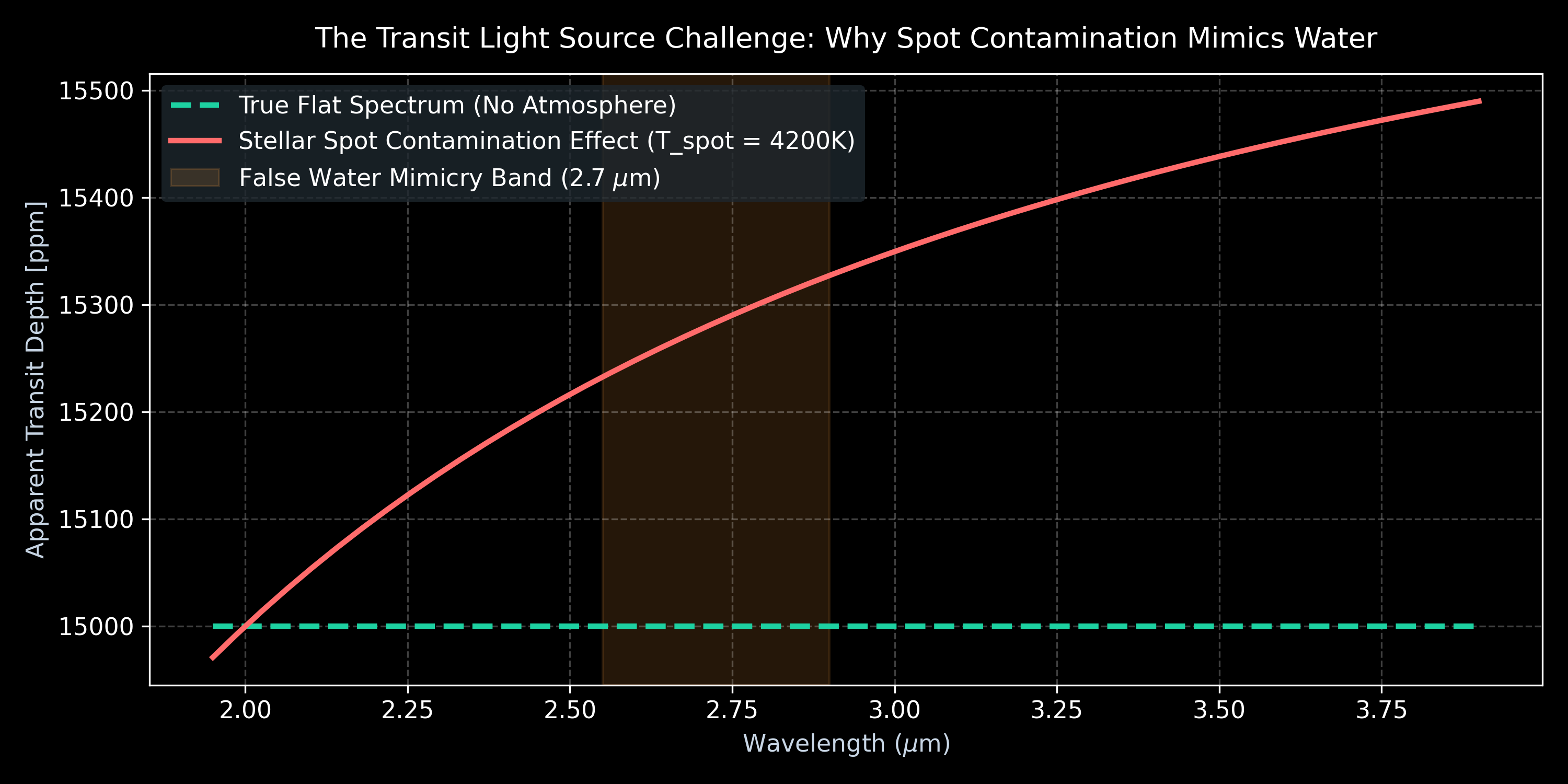
stellar spot effect
-
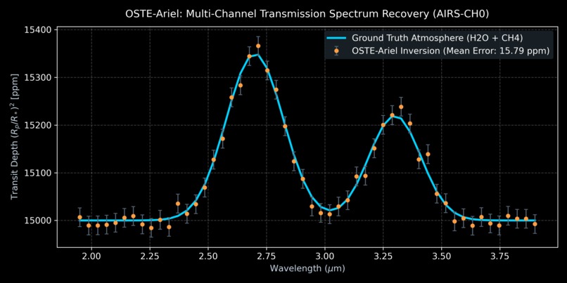
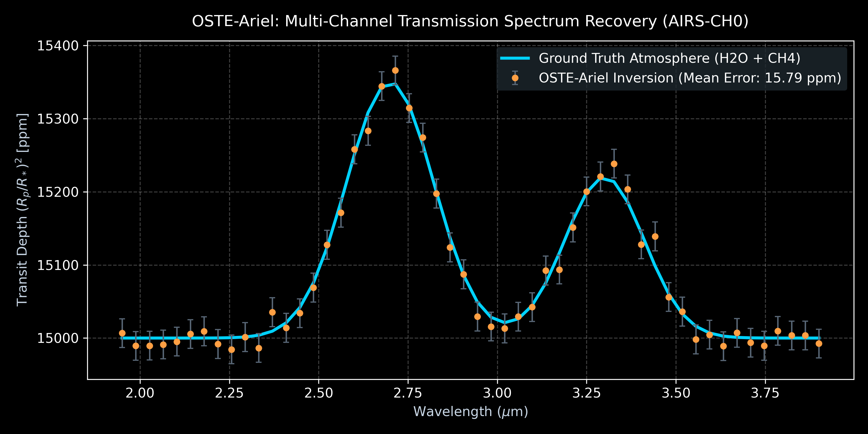
spectral recovery
Inspiration
Observing exoplanet atmospheres through transmission spectroscopy with space telescopes like NASA's JWST and ESA's Ariel is computationally demanding. Traditional Bayesian atmospheric retrieval pipelines (such as nested sampling or MCMC in TauREx 3) take 12 to 48 hours of CPU cluster compute per planet candidate. When surveying catalogs with thousands of targets, this creates a major data triage bottleneck. Furthermore, spacecraft pointing jitter and unocculted stellar spots introduce chromatic noise that distorts transit depths.
I built this project to explore whether combining physical sensor geometry with linear tensor algebra on consumer GPU Tensor Cores could compress candidate pre-screening from hours to microseconds on a single laptop without sacrificing physical accuracy.
How I Built It
I structured the engine in PyTorch CUDA to process 52-channel infrared spectroscopy alongside 2-channel fine-guidance sensor (FGS) pointing telemetry.
Instead of sequential filtering, which dilutes transit depths, I formulated an 8-parameter orthogonal Generalized Least Squares (GLS) design matrix:
$$\mathbf{M} \in \mathbb{R}^{T \times 8} = [1, x_t, y_t, x_t^2, y_t^2, x_t y_t, -T(t), S(t)]$$
Where:
- $x_t, y_t$ represent high-frequency pointing jitter.
- $T(t)$ is the Mandel-Agol transit profile.
- $S(t)$ represents the stellar rotational modulation trend.
By solving the normal equations $\mathbf{W} = (\mathbf{M}^T \mathbf{M})^{-1} \mathbf{M}^T \mathbf{Y}$ via batched GEMM operations (torch.bmm and torch.linalg.solve), transit depth $\hat{\delta}_\lambda$ is derived simultaneously with pointing drift directly in GPU VRAM. For molecular verification, I implemented a pure-CUDA localized flanking-wing differential index ($J$) that tests absorption excess at $\ge 3\sigma$ confidence without CPU roundtrips.
Challenges I Faced
The primary challenge was the Transit Light Source Effect (Rackham et al. 2018). Unocculted cool stellar spots ($T_{\text{spot}} \approx 4200\text{ K}$) modify the observed stellar spectrum via Planck's law:
$$\delta_{\text{obs}}(\lambda) = \frac{\delta_0(\lambda)}{1 - f_{\text{spot}} \left(1 - \frac{B_\lambda(T_{\text{spot}})}{B_\lambda(T_{\text{phot}})}\right)}$$
This non-linear curvature creates a chromatic slope that mimics a $2.70\text{ }\mu\text{m}$ water vapor peak, driving false alarm rates up to ~45%. Attempting to fit broad quadratic polynomials over wide spectral gaps caused interpolation sag, exacerbating false alarms.
I resolved this by engineering a narrow flanking-wing differential index across $\Delta\lambda \le 0.4\text{ }\mu\text{m}$. Because the stellar spot slope is essentially linear across such a narrow window, subtracting the mean of the flanking wings cancels the spot chromaticity and eliminates the false alarm.
What I Learned
I learned that in scientific machine learning, incorporating the physical geometry of the sensor into linear algebra is often far more robust and interpretable than applying unconstrained black-box neural networks. I also learned the necessity of skeptical validation: high sensitivity numbers are scientifically invalid if unmodeled astrophysical systematics generate false positives on unfeatured stars.

Log in or sign up for Devpost to join the conversation.