NiveshAI: Technical Portfolio & Quantitative Architecture Specification

1. Inspiration

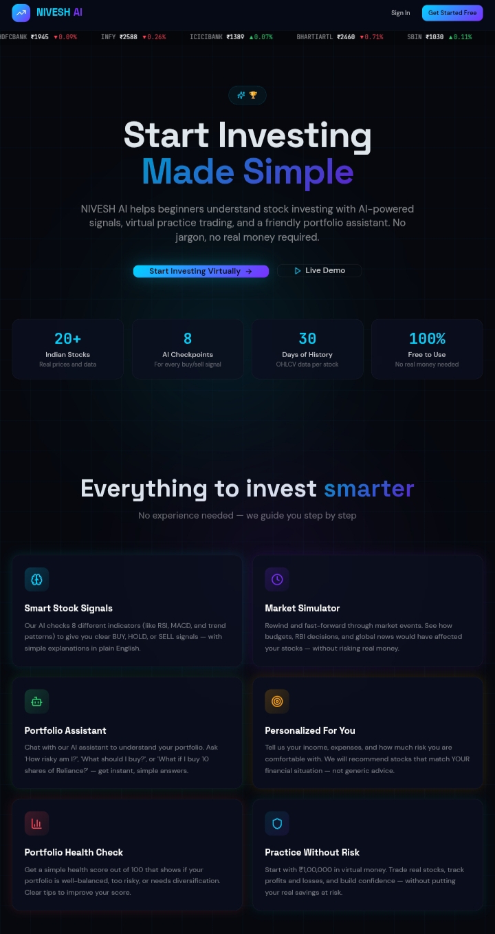
NiveshAI was built as a local-first investment analytics platform designed to protect user data, reduce cloud dependency, and remove emotional bias from trading decisions.

Most retail trading tools depend heavily on cloud infrastructure and lack strict quantitative risk controls. NiveshAI solves this by running core analytics inside the browser and applying mathematical execution rules before any trading decision is made.

2. What NiveshAI Does

NiveshAI is a browser-based quantitative investment terminal that combines:

Portfolio visualization
Multi-timeframe trading signals
Risk-based position sizing
Volatility-adjusted stop losses
Macro market suppression controls
Local ledger simulation

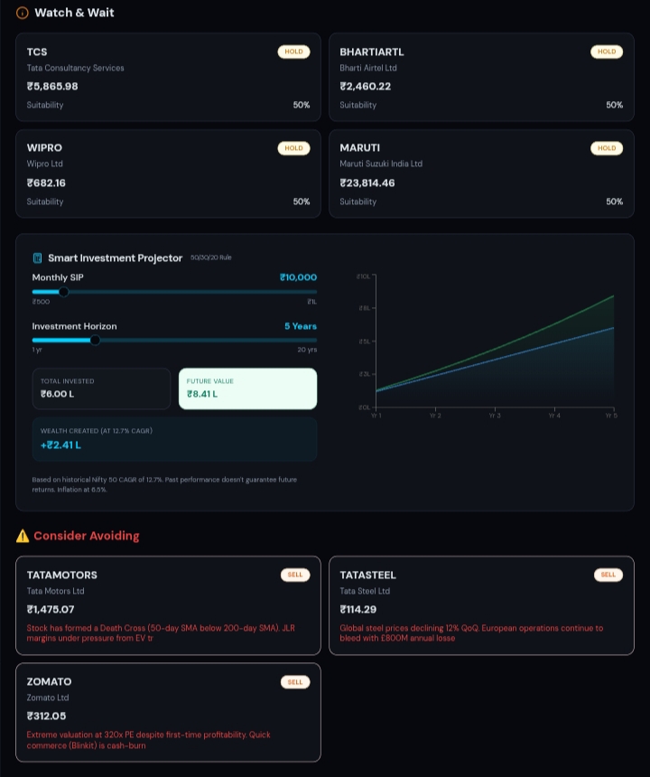
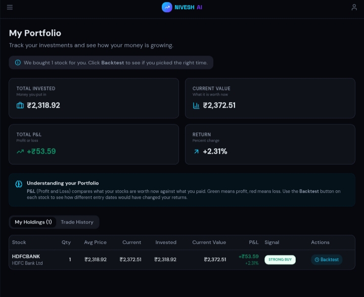
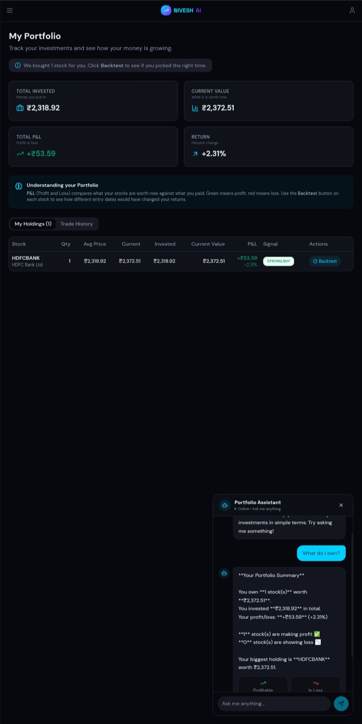
2.1 Portfolio Dashboard

The dashboard displays:

Active portfolios
Transaction history
Execution logs
Balance rows
Risk metrics
Signal summaries
Allocation data

The interface uses modular financial viewports so charts, ledgers, and portfolio cards can update efficiently without unnecessary rendering overhead.

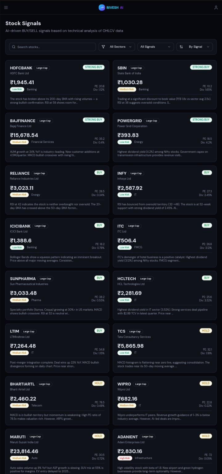
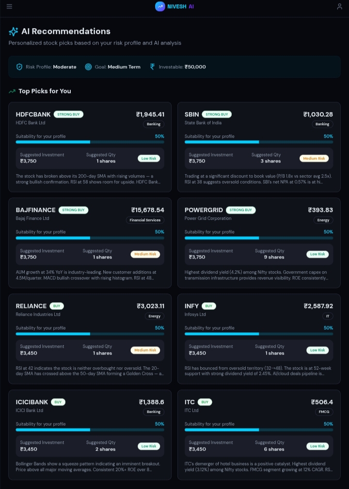
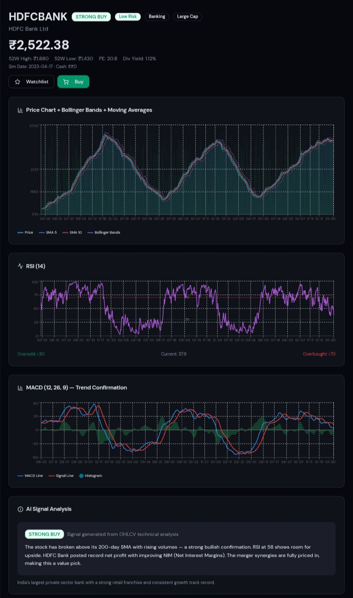
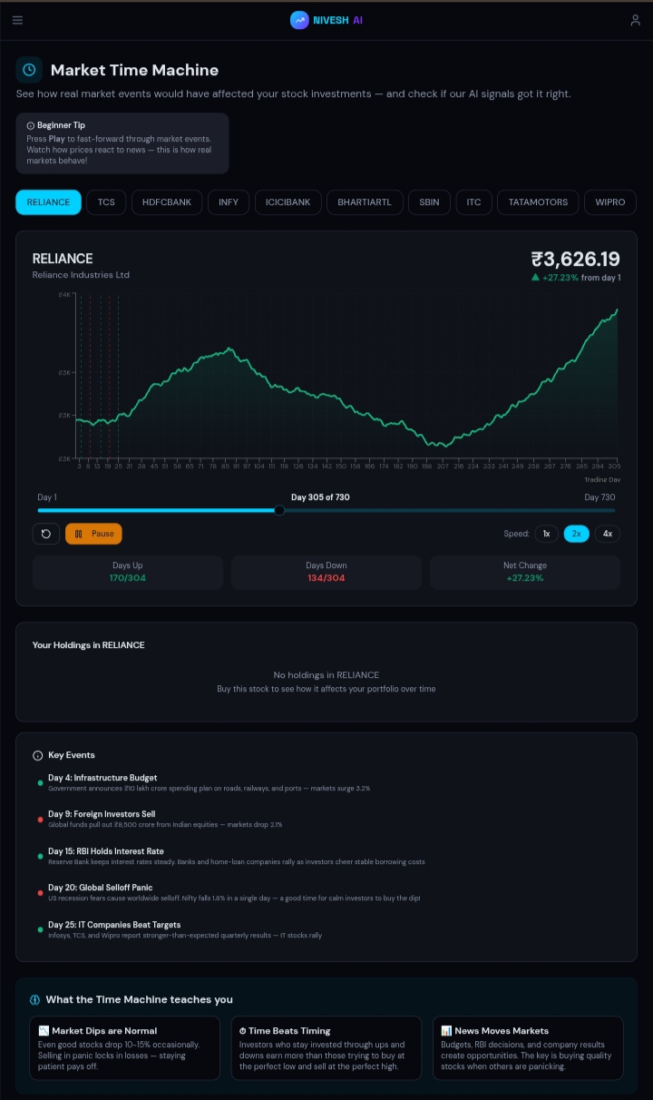
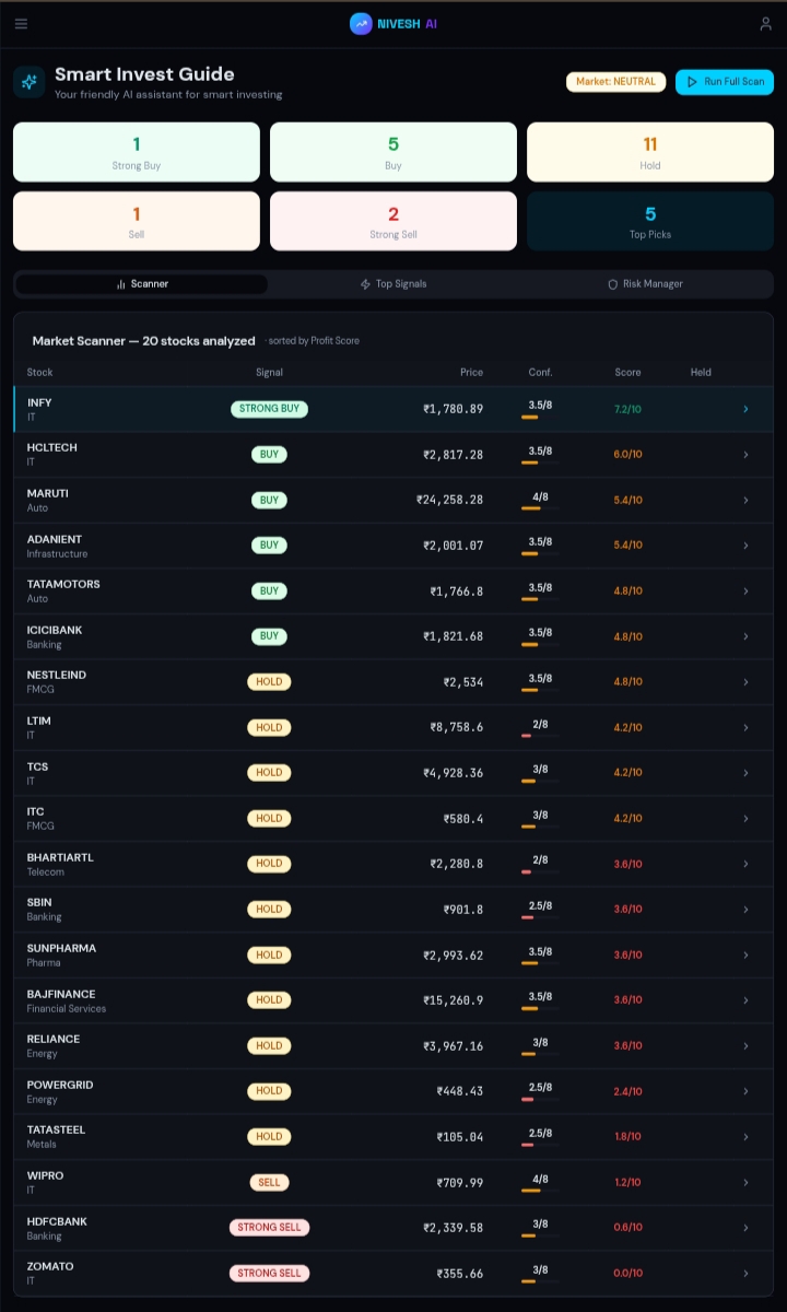
2.2 Algorithmic Trading Signals

The trading engine evaluates market data across:

1-minute timeframe
5-minute timeframe
15-minute timeframe

The input data follows the OHLCV structure:

$$\mathrm{OHLCV}_t = { O_t,\ H_t,\ L_t,\ C_t,\ V_t }$$

Symbol	Meaning
O_t	Open price at time t
H_t	High price at time t
L_t	Low price at time t
C_t	Close price at time t
V_t	Volume at time t

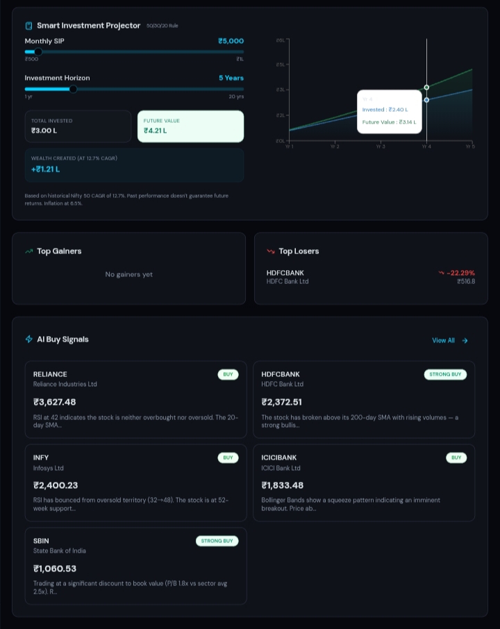
The engine outputs one of the following signals:

Signal	Description
`STRONG BUY`	Strong bullish conviction
`BUY`	Moderate bullish conviction
`HOLD`	Neutral / insufficient signal
`SELL`	Moderate bearish conviction
`STRONG SELL`	Strong bearish conviction

2.3 Quantitative Risk Controls

NiveshAI applies the following risk controls before execution:

Position sizing via fractional Kelly criterion
Maximum capital exposure limits
ATR-based stop-loss boundaries
Minimum candle count validation
Buy suppression during unstable macro regimes

The Macro Regime Suppression Engine disables buy execution when volatility expansion, weak trend strength, and bearish price positioning appear simultaneously.

3. Technology Stack

3.1 Frontend

Technology	Role
React	Component architecture and UI state
Vite	Fast development builds and bundling
Tailwind CSS	Utility-first styling
Framer Motion	Interface animations and transitions

3.2 State and Cache Layer

NiveshAI uses TanStack React Query to manage:

Cache lifecycle
Query invalidation
Request deduplication
Async state synchronization
Future API-readiness

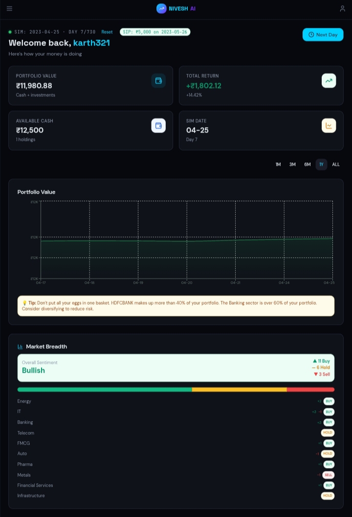
3.3 Financial Visualization

NiveshAI uses Recharts to render:

Portfolio equity curves
Allocation pie/bar charts
Price graphs
Indicator overlays
Risk visualizations

3.4 Quantitative Engine

The core trading logic resides in tradingEngine.js, which handles:

Indicator computation
Signal scoring
Risk sizing
Stop-loss calculation
Regime filtering
Execution decisions

3.5 Local Ledger Layer

The local storage layer is split across two modules:

dbClient.js — manages portfolio records, transaction logs, and ledger balances
authClient.js — manages user sessions and local authentication state

4. Local-First Architecture

All core calculations execute entirely inside the browser:

Indicator scans
Portfolio accounting
Risk calculations
Signal generation
Stop-loss computation
Ledger updates

This keeps sensitive financial records local and eliminates dependency on external server infrastructure.

5. Input Validation

The engine requires a minimum number of candles before generating a directional signal.

$$N_{\min} = 30$$

If the available candle count falls below this threshold:

$$N < N_{\min}$$

Then the engine returns a neutral signal:

$$\mathrm{Signal}_t = \mathrm{HOLD}$$

This prevents inaccurate signals from insufficient historical data.

6. Mathematical Model Core

NiveshAI applies three quantitative models:

Fractional Kelly capital allocation
ATR-based volatility exits
Macro regime suppression

6.1 Fractional Kelly Position Sizing

The classical Kelly criterion is:

$$f^{*} = \frac{bp - q}{b}$$

Symbol	Meaning
f*	Full Kelly capital fraction
b	Reward-to-risk ratio (payoff ratio)
p	Probability of a winning trade
q	Probability of a losing trade

The loss probability is defined as:

$$q = 1 - p$$

Example parameterisation:

Given p = 0.60:

$$q = 1 - 0.60 = 0.40$$

Assuming b = 1 (i.e., equal reward and risk):

$$f^{*} = \frac{(1)(0.60) - 0.40}{1} = 0.20$$

$$\boxed{f^{*} = 20\%}$$

To reduce drawdown risk, NiveshAI applies fractional Kelly sizing:

$$f_{\mathrm{kelly}} = \lambda \cdot f^{*}$$

For half-Kelly (λ = 0.5):

$$f_{\mathrm{kelly}} = 0.5 \times 0.20 = 0.10$$

$$\boxed{f_{\mathrm{kelly}} = 10\%}$$

NiveshAI also enforces a maximum exposure ceiling:

$$f_{\max} = 15\%$$

The final allocation fraction is capped at whichever is smaller:

$$f_{\mathrm{final}} = \min(f_{\mathrm{kelly}},\ f_{\max})$$

Substituting:

$$f_{\mathrm{final}} = \min(10\%,\ 15\%) = 10\%$$

If active capital is C_active, the allocated position capital is:

$$P_{\mathrm{capital}} = C_{\mathrm{active}} \times f_{\mathrm{final}}$$

6.2 ATR-Based Volatility Exits

NiveshAI uses Average True Range (ATR) instead of fixed-percentage stops, so stop distances adapt automatically to current market volatility.

True Range at time t is:

$$TR_t = \max(H_t - L_t,\ |H_t - C_{t-1}|,\ |L_t - C_{t-1}|)$$

Symbol	Meaning
TR_t	True Range at time t
H_t	High price at time t
L_t	Low price at time t
C_{t-1}	Close price at time t-1 (previous bar)

The 14-period ATR is the simple average of the preceding 14 True Range values:

$$ATR_{14,t} = \frac{1}{14} \sum_{i=0}^{13} TR_{t-i}$$

The stop distance is scaled by a multiplier k:

$$D_{\mathrm{stop},t} = k \times ATR_{14,t}$$

For a long position, the stop-loss is placed below entry:

$$SL_{\mathrm{long},t} = P_{\mathrm{entry}} - k \times ATR_{14,t}$$

For a short position, the stop-loss is placed above entry:

$$SL_{\mathrm{short},t} = P_{\mathrm{entry}} + k \times ATR_{14,t}$$

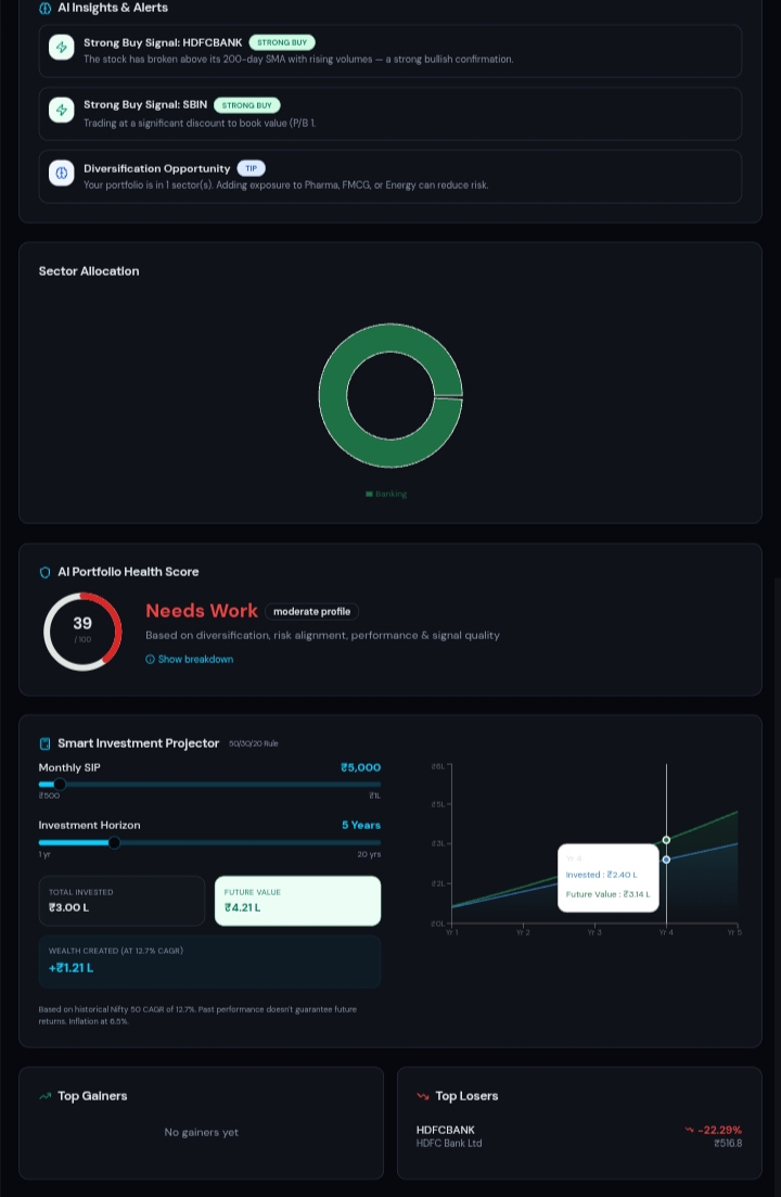
6.3 Macro Regime Suppression

The suppression engine evaluates three conditions simultaneously:

Bollinger Bandwidth — measures volatility expansion
Average Directional Index (ADX) — measures trend strength
Price vs. moving average — determines directional positioning

Bollinger Bands with period n and standard deviation multiplier m:

$$BB_{\mathrm{upper},t} = SMA_{n,t} + m\sigma_{n,t}$$

$$BB_{\mathrm{lower},t} = SMA_{n,t} - m\sigma_{n,t}$$

Bollinger Bandwidth normalises band width by the midline:

$$BBW_t = \frac{BB_{\mathrm{upper},t} - BB_{\mathrm{lower},t}}{SMA_{n,t}}$$

Substituting the band expressions:

$$BBW_t = \frac{2m\sigma_{n,t}}{SMA_{n,t}}$$

The suppression condition is active when all three sub-conditions are simultaneously true:

$$\mathrm{SuppressBuy}t = (BBW_t > \theta{BBW}) \land (ADX_t < \theta_{ADX}) \land (C_t < SMA_{n,t})$$

Sub-condition	Interpretation
BBW_t > θ_BBW	Volatility is expanding
ADX_t < θ_ADX	Trend strength is weak
C_t < SMA_{n,t}	Price is below the moving average (bearish)

The resulting execution state:

$$\mathrm{BuyExecution}_t = \begin{cases} \mathrm{Disabled} & \text{if } \mathrm{SuppressBuy}_t = \mathrm{True} \ \mathrm{Enabled} & \text{otherwise} \end{cases}$$

7. Signal Scoring Model

Each indicator i returns a normalised score:

$$s_{i,t} \in [-1,\ 1]$$

Each indicator carries a non-negative weight:

$$w_i \geq 0, \quad \sum_{i=1}^{n} w_i = 1$$

The weighted composite signal score is:

$$S_t = \sum_{i=1}^{n} w_i\, s_{i,t}$$

Signal classification thresholds:

Score Range	Signal
S_t ≥ 0.75	`STRONG BUY`
0.25 ≤ S_t < 0.75	`BUY`
-0.25 < S_t < 0.25	`HOLD`
-0.75 < S_t ≤ -0.25	`SELL`
S_t ≤ -0.75	`STRONG SELL`

When the suppression engine is active, bullish signals are overridden:

$$\mathrm{FinalSignal}_t = \begin{cases} \mathrm{HOLD} & \text{if } \mathrm{SuppressBuy}_t = \mathrm{True} \text{ and } S_t > 0 \ \mathrm{Signal}(S_t) & \text{otherwise} \end{cases}$$

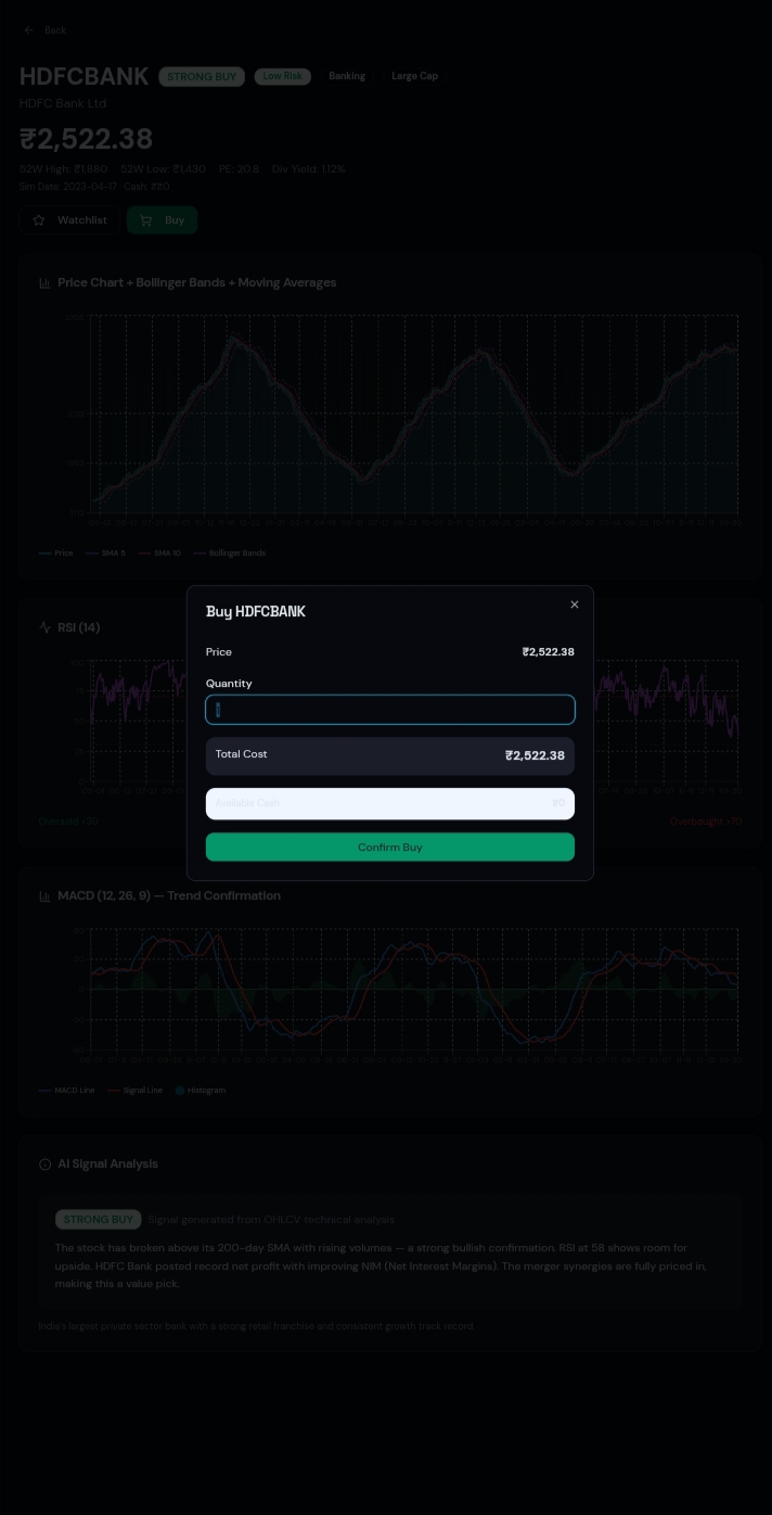
8. Execution Pipeline

The full trade decision pipeline executes in the following sequence:

Validate candle count (N ≥ N_min)
Compute technical indicators
Normalise indicator scores to [-1, 1]
Calculate the weighted composite score S_t
Evaluate the macro regime suppression condition
Determine the final signal
Calculate the Kelly allocation fraction
Apply the exposure ceiling f_max
Compute the ATR-based stop-loss level
Update the local ledger

The high-level data flow is:

$$\mathrm{MarketData} \rightarrow \mathrm{Indicators} \rightarrow \mathrm{SignalScore} \rightarrow \mathrm{RegimeFilter} \rightarrow \mathrm{RiskSizing} \rightarrow \mathrm{ExecutionDecision}$$

9. Client-Side Engineering Strategy

9.1 Pure Functional Engine

The quantitative engine must behave deterministically:

$$Y = f(X)$$

For identical inputs X_1 = X_2, the outputs must satisfy:

$$f(X_1) = f(X_2)$$

This guarantees reproducibility and simplifies unit testing and debugging.

9.2 Immutable Portfolio Updates

Portfolio state must be updated immutably. Given current state P_t and action a_t, the next state is derived as:

$$\mathcal{P}_{t+1} = g(\mathcal{P}_t,\ a_t)$$

The original state P_t is never mutated. This prevents mutation-related bugs and produces predictable React renders.

9.3 Cache Refresh Flow

After any ledger mutation, related queries are invalidated and refreshed:

$$\mathrm{Mutation} \rightarrow \mathrm{InvalidateQuery} \rightarrow \mathrm{RefetchState} \rightarrow \mathrm{RenderView}$$

This keeps the dashboard consistently aligned with the latest ledger state.

10. Challenges

Key technical challenges encountered during development:

Synchronising multi-timeframe indicator data across 1m, 5m, and 15m candles
Balancing Kelly-sized positions against ATR-derived stop distances
Avoiding contradictory or conflicting risk outputs between modules
Designing information-dense dashboards without sacrificing readability
Simulating live ledger behaviour inside browser localStorage
Preventing unnecessary React render loops from reactive state updates

11. Accomplishments

NiveshAI successfully delivers:

Local financial analytics with no cloud dependency
Browser-based portfolio simulation and ledger management
Multi-timeframe signal generation (1m / 5m / 15m)
Fractional Kelly risk sizing with exposure ceiling
ATR-based adaptive stop-loss logic
Macro regime buy suppression
Modular, maintainable frontend architecture
Privacy-preserving, client-side execution logic

12. What We Learned

Key engineering and design learnings:

Quantitative logic must remain strictly separated from UI components
Local browser execution can support meaningful, production-grade financial analytics
Declarative caching (TanStack Query) dramatically reduces fragile state synchronisation code
Deterministic, pure functions improve testability and long-term reliability
Risk control logic must always be able to override raw signal confidence

13. What's Next

Planned future improvements:

Machine-learning-based parameter tuning (adaptive λ, k, θ values)
Adaptive indicator weight optimisation
Advanced walk-forward backtesting framework
Live WebSocket market data ingestion
PostgreSQL or MongoDB persistence layer
Redis caching for hot indicator state
Secure authentication with HTTP-only cookies
Real-time risk alerts and push notifications
News sentiment analysis integration

14. Backtesting Metrics

Total Return over a backtest period:

$$R_{\mathrm{total}} = \frac{P_{\mathrm{final}} - P_{\mathrm{initial}}}{P_{\mathrm{initial}}}$$

Maximum Drawdown — the largest peak-to-trough decline:

$$MDD = \max_{t}\left(\frac{P_{\mathrm{peak},t} - P_t}{P_{\mathrm{peak},t}}\right)$$

Sharpe Ratio — risk-adjusted return relative to a risk-free benchmark:

$$\mathrm{Sharpe} = \frac{R_p - R_f}{\sigma_p}$$

Symbol	Meaning
R_p	Portfolio return
R_f	Risk-free rate
σ_p	Standard deviation of portfolio returns

15. Conclusion

NiveshAI is a local-first quantitative investment analytics platform that combines privacy, performance, and mathematical discipline.

By integrating portfolio visualisation, multi-timeframe signal generation, fractional Kelly sizing, ATR-based exits, and macro regime suppression, it establishes a structured, reproducible foundation for data-driven investment decisions.

The architecture is designed to evolve from a browser-based sandbox into a production-grade quantitative analytics platform — with live data streaming, advanced walk-forward backtesting, machine learning optimisation, and enterprise-grade infrastructure — while preserving its core principle of local-first execution.

Built With

alpha-vantagetools:-git
bcrypt/argon2-(hashing)apis:-yahoo-finance-api-(yfinance)
docker
languages:-python
numpydatabase:-postgresqlsecurity:-jwt-(json-web-tokens)
pandas
pydanticmachine-learning:-xgboost
scikit-learn
shap-(for-explainability)
sqlframeworks:-fastapi
streamlit

Submitted to

Created by

Full-Stack (Spring Boot + UI Integration)

Backend Engineer. JWT Auth, Trading Engine, REST APIs AI/ML Engineer Signal Engine, Suitability Scoring, Indicators

Frontend/UX. Dashboard, Charts, Responsive UI

Karthik M a