-
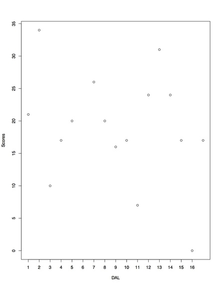
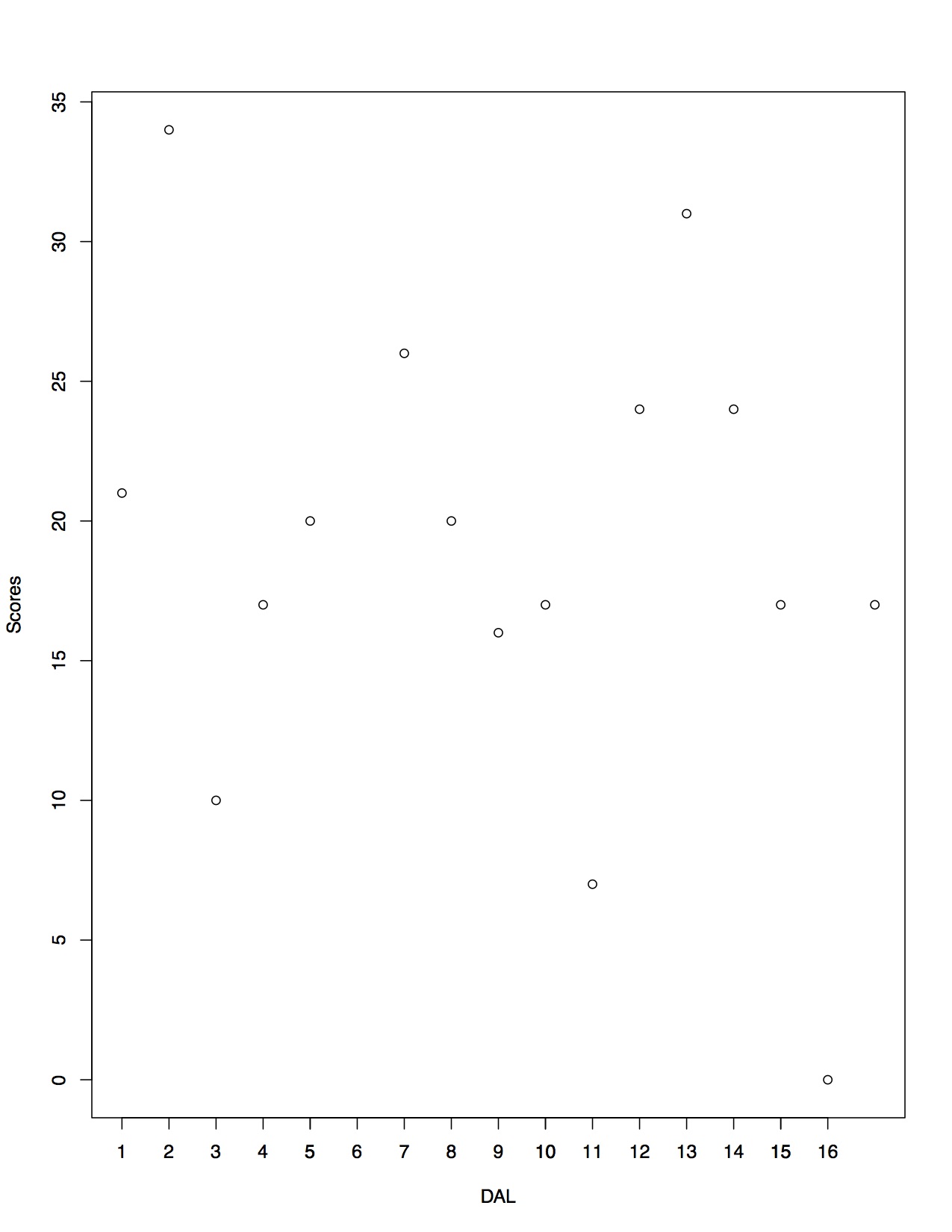
Fig 1: Scores for DAL 2009 regular season
-
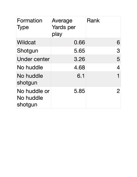
Fig 2: AYP v.s Formation 2019 regular season
-
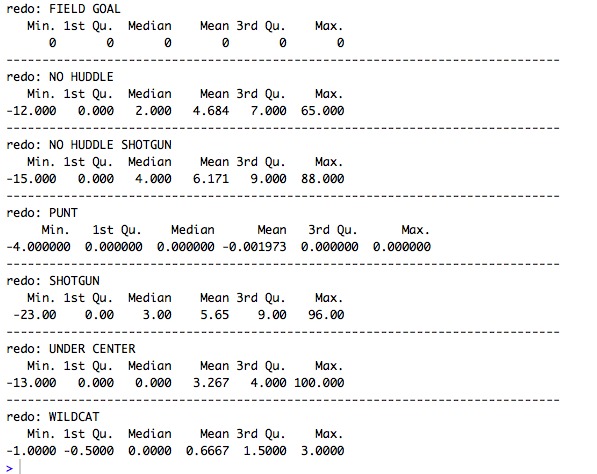
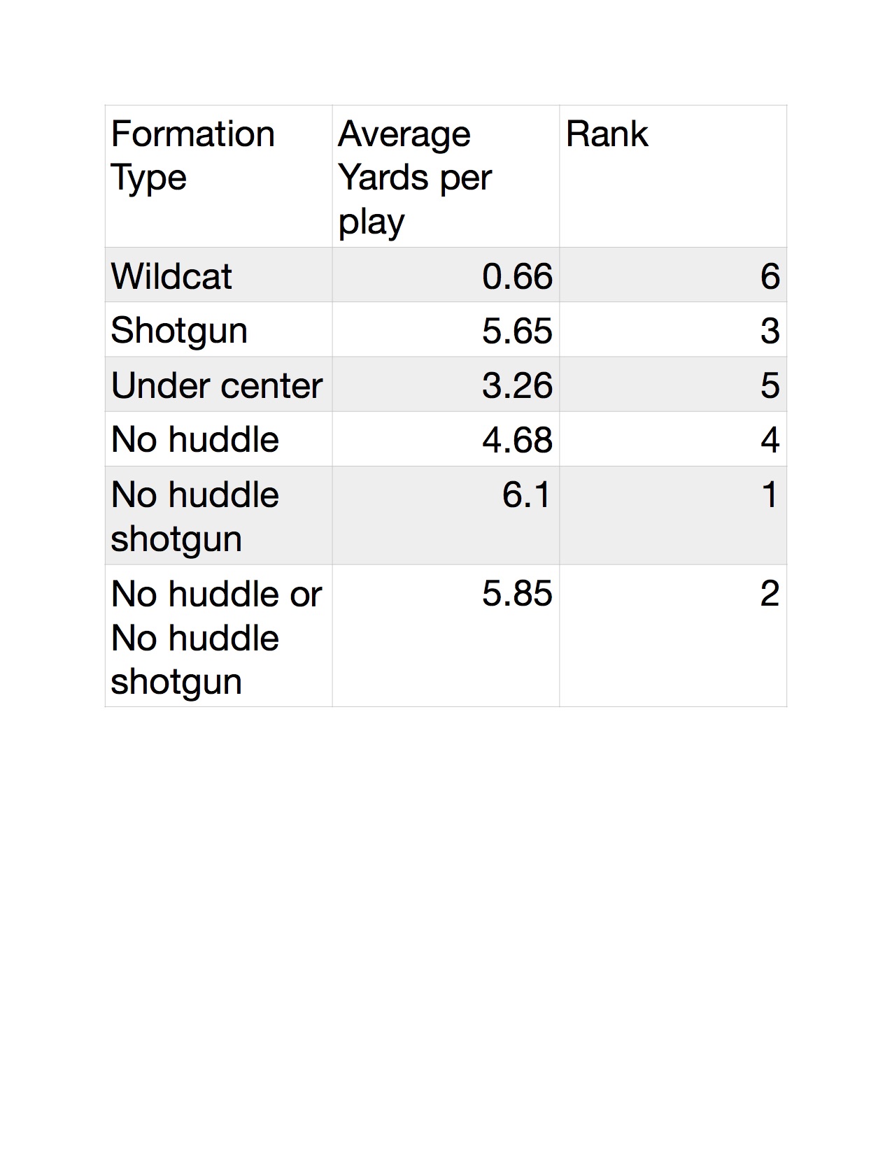
Fig.3 Summary of Data: AYP v.s Formation ('18-'19 Reg Season)
-

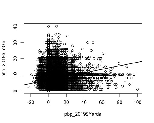
Fig 4. Simple Regression for Yards to Go v.s Yards
-

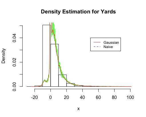
Fig.5 Density Estimation for Yards Distribution

A short project detailing some of the skills I learned in r while analyzing NFL data sets; see https://github.com/ryurko for more details on obtaining the data. I obtained play-by-play data from NFLsavant; http://nflsavant.com/about.php.
So far I've been working on manipulating the data; here I've taken 4 columns of the data (home team, away team, away score, home score) and plotted them to see all of the scores for the Dallas Cowboys over the 2009 regular season. (Fig 1)
Next I wanted to test a theory I've had from playing Madden all these years. I manipulated 2019 NFL play-by-play data and computed the average yards per plan for each formation to answer the following question: Does a no-huddle offence catch the defence by surprise- leading to more yardage? Unsurprisingly the answer is yes; however interestingly enough we see that if we run a no-huddle formation under center; the average yard per play (AYP) is still lower than if we ran the play under the shotgun formation. Hence, the 'best' formation would be to run No huddle offence under shotgun (obviously impossible to do the entire game). (Fig 2)
Here I'm just showing more complete results after fig 2. I worked on making a more efficient code and I'm just showing the summary of the data of the formations. I also added the 2018 reg season data for a more reliable sample. I removed some bad data (104 Yrds on a fumble return for example). Recall 50% of the data falls between the first and 3rd quartile. What's unfortunate is this data does not account for play action-or else why would anyone run a play under center? (fig 3)
I preformed some simple regression; unfortunately the data is such that logistic regression would make alot more sense (there is very little continuous data, most columns are discrete indicators). I thought I'd compared how many "Yards to Go" i.e the distance from the first down marker (ToGo) an offence had, compared to the total yards completed in that play (Yards). The line of fit isn't great because the graph shows the data is clearly bi-modal. (Fig.4)
For my next contribution, I decided to try some basic density estimation techniques. I plotted a histogram of the "Yards" data, and used a naive and guassian estimated. Since the data is bimodel, the estimators do pretty well at the tails of the data, but is clearly terrible near the mean. (fig. 5)
The end goal would be building a win simple projection system for the 2020 season.
Update: check out https://www.kaggle.com/sportsstatseli/nba-boxscore-regression for a few simple regression models using NBA boxscore data. Due to the poorness of the NFL data that I've been able to find I've been working with different data sets; when I have new results I will either post them here or provide another link to the new kaggle/devpost page.


Log in or sign up for Devpost to join the conversation.