-

NeuroStack thumbnail
-
PCA scatter plot

Inspiration
Alzheimer’s is one of those problems that sits right at the intersection of deeply human and deeply technical. I normally work on cybersecurity and ML pipelines (e.g., phishing detection, threat intelligence), and I kept noticing that those same ideas—multi-source data, anomaly detection, ensemble models—could be repurposed for something that actually touches people’s lives.
Around the same time, a close friend told me about their grandmother’s experience with Alzheimer’s. That made this hackathon feel less like a “toy” project and more like a chance to prototype something meaningful: could I take my skills with pipelines and modeling and build a small, reproducible system for early Alzheimer’s risk detection?
That’s where this project came from.
What it does
This project is a multi-view ensemble model for early Alzheimer’s risk detection using two complementary, tabular datasets derived from the same OASIS cohort:
Dataset A – Alzheimer Features (clinical view)
Columns likeAge,EDUC,SES,MMSE,CDR,eTIV,nWBV,ASF, and the labelGroup(Nondemented,Demented,Converted).Dataset B – Dementia/OASIS (clinical + MRI metadata view)
The same population with extra metadata such asSubject ID,MRI ID,Visit,MR Delay,Hand, plus the same clinical / volumetric features and the sameGrouplabels.
I reformulated the task as a binary classification problem:
- Non-impaired:
Nondemented - Impaired:
DementedorConverted
For each dataset separately, I trained a model zoo and then a stacking ensemble:
- Logistic Regression (baseline, interpretable model)
- RandomForestClassifier
- XGBoost (XGBClassifier)
- LightGBM (LGBMClassifier)
- StackingClassifier with RF + XGBoost + LightGBM as base learners and Logistic Regression as the meta-learner
On held-out test sets, the final stacking ensemble achieves roughly:
Dataset A (Alzheimer Features – clinical view):
- Test accuracy ≈ 95%
- Test ROC AUC ≈ 0.95
Dataset B (Dementia/OASIS – clinical + MRI view):
- Test accuracy ≈ 95%
- Test ROC AUC ≈ 0.96
So the system can reliably distinguish “non-impaired” vs “impaired” individuals using only basic clinical and structural brain volume features.
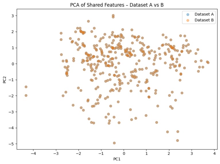
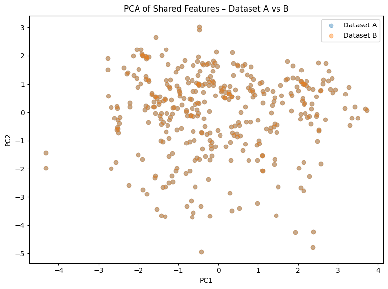
To understand how similar the two views really are, I also do an unsupervised analysis of the shared feature space using PCA. I take the 8 features shared by both datasets:
ASF,Age,CDR,EDUC,MMSE,SES,eTIV,nWBV
Then I scale them jointly, run PCA to 2D, and visualize Dataset A vs Dataset B in this latent space. This shows how both datasets occupy similar regions in the shared feature manifold and supports treating them as consistent views of the same underlying biology.
How I built it
Data loading and organization
- Mounted Google Drive in Google Colab.
- Stored everything inside a project folder
alzh/with:data/alzheimer.csv(Dataset A – Alzheimer Features)data/dementia.csv(Dataset B – Dementia/OASIS)
- Wrote a reusable
load_tabular_datasethelper to:- Read the CSV
- Drop non-numeric columns (e.g.,
M/F,Subject ID,MRI ID,Hand) - Split into train / validation / test (70% / 15% / 15%)
- Impute missing values with median imputation
- Standardize features with StandardScaler
Label engineering
- Source label:
Group ∈ {Nondemented, Demented, Converted}. - New binary label:
0→Nondemented(non-impaired)1→DementedorConverted(impaired / at risk)
- Verified that both training sets are reasonably balanced (roughly half non-impaired, half impaired).
- Source label:
Model zoo per dataset
- For both Dataset A and Dataset B, I trained the following models:
- Logistic Regression (L2-regularized)
- RandomForestClassifier
- XGBClassifier
- LGBMClassifier
- All models are evaluated on the validation set with:
- Accuracy
- Precision, recall, F1
- ROC AUC (binary classification)
- For both Dataset A and Dataset B, I trained the following models:
Stacking ensemble
- For each dataset, I constructed a StackingClassifier:
- Base estimators: RandomForest, XGBoost, LightGBM
- Final meta-learner: Logistic Regression
- Training procedure:
- Train models on the training split
- Evaluate on the validation split
- Then refit the stacking ensemble on train + validation
- Evaluate final performance on the held-out test set
- This gives the final reported accuracy and ROC AUC for each dataset.
- For each dataset, I constructed a StackingClassifier:
Unsupervised shared-feature analysis (PCA)
- Computed the intersection of feature names between Dataset A and Dataset B.
- Found 8 shared features (
ASF,Age,CDR,EDUC,MMSE,SES,eTIV,nWBV). - Combined both datasets in this shared feature space, scaled them, and applied PCA → 2D.
- Plotted Dataset A vs Dataset B points, and inspected the explained variance ratios for PC1 and PC2.
- This acts as an unsupervised “sanity check” that the two datasets are aligned and that treating them as multiple views is reasonable.
Explainability and what I learned
While this isn’t a full SHAP/LIME dashboard, I tried to keep the system interpretable:
- The core features are clinically meaningful: cognitive scores (MMSE, CDR), education, socioeconomic status, and structural brain volume measures (eTIV, nWBV, ASF).
- I used Logistic Regression and tree-based models, which naturally expose feature importances or coefficients.
- I used PCA on shared features to visualize how the two datasets align and to understand the structure of the feature space.
From this project, I learned:
- How to treat clinical features and MRI-derived volumetric features as multiple views of the same problem, the same way I think about multi-source data in threat intelligence.
- How to build a robust, reproducible ML pipeline that:
- Loads real-world biomedical data from multiple sources,
- Handles missing values safely,
- Trains several classical models,
- Uses stacking to get stable performance,
- And evaluates on a truly unseen test set.
- How to use unsupervised methods (PCA) to reason about dataset consistency, not just model metrics.
Challenges
- Data & environment debugging:
There were a lot of path / mounting / CSV issues to chase down in Colab before the pipeline was stable. - NaNs & preprocessing:
Some columns likeSEScontained missing values. Early versions of the models crashed until I integrated median imputation and kept it consistent across train/val/test. - Small dataset vs overfitting:
With only ~373 rows, it’s tempting to over-tune models. I constrained myself to simple, classical models and a clean train/val/test structure to avoid “leaderboard overfitting.” - Framing the label:
I had to decide what to do with theConvertedclass. For hackathon scope, I folded it into “impaired” to get a clinically meaningful binary label, and left progression modeling as future work.
What’s next
If I extend this project after the hackathon, I’d like to:
- Model progression risk explicitly (e.g., probability that a
Nondementedsubject will convert over time). - Add calibrated risk scores and stronger explainability (e.g., SHAP values, partial dependence plots) so that clinicians can see why the model is making its predictions.
- Integrate additional open datasets (e.g., speech or longitudinal cognitive assessments) using the same multi-view ensemble idea.
Even though this is “just” a hackathon project, my goal was to build a serious, end-to-end pipeline that other students and researchers could reproduce, remix, and improve as they explore AI for Alzheimer’s.
Built With
- jupyter-notebook
- lightgbm
- numpy
- pandas
- python
- scikit-learn
- xgboost


Log in or sign up for Devpost to join the conversation.