-
-
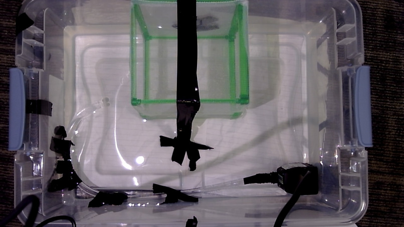
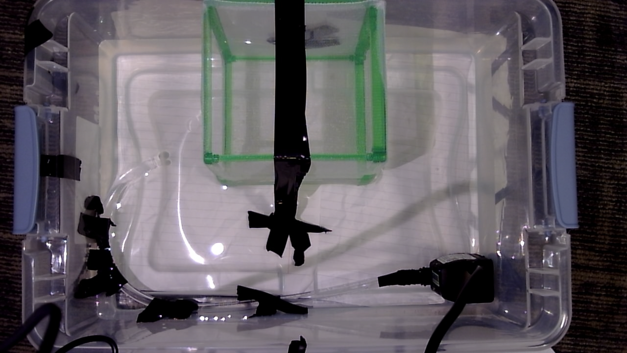
01. Real prototype: C270 webcam, tray, pump, tubing, green marker and mesh collector. Pump power is manual.
-
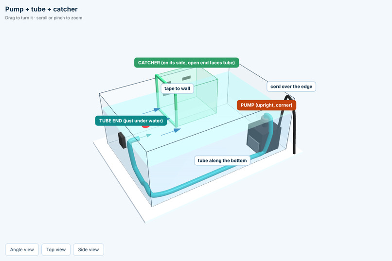
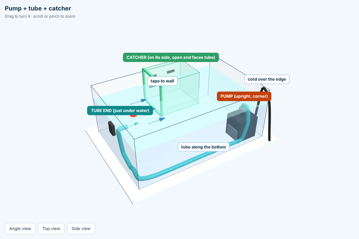
02. Pump, tubing and mesh catcher. Illustrative hardware layout; arrows show intended circulation, not measured flow.
-
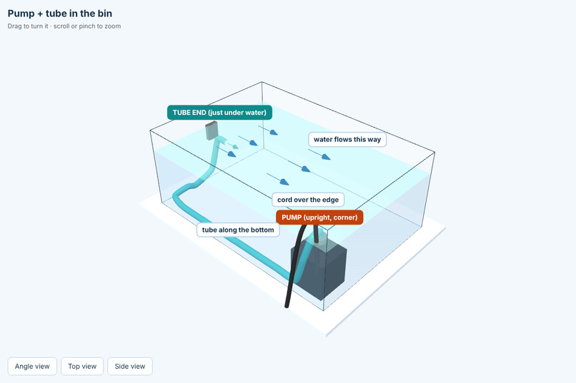
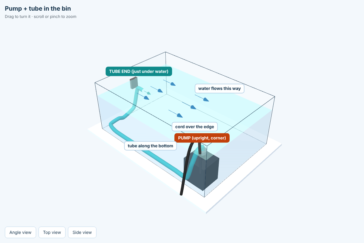
03. Pump and tubing routing inside the tray. Schematic illustration of the return outlet and intended flow direction.
-
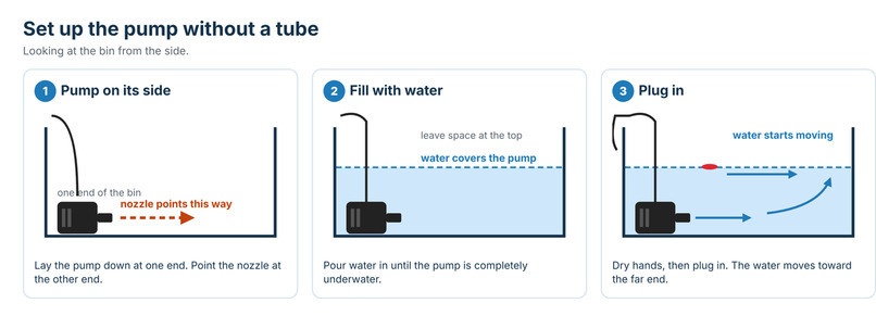
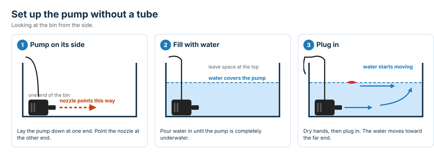
04. Alternative setup without tubing. Pump orientation differs from the tubing configuration shown above.
-
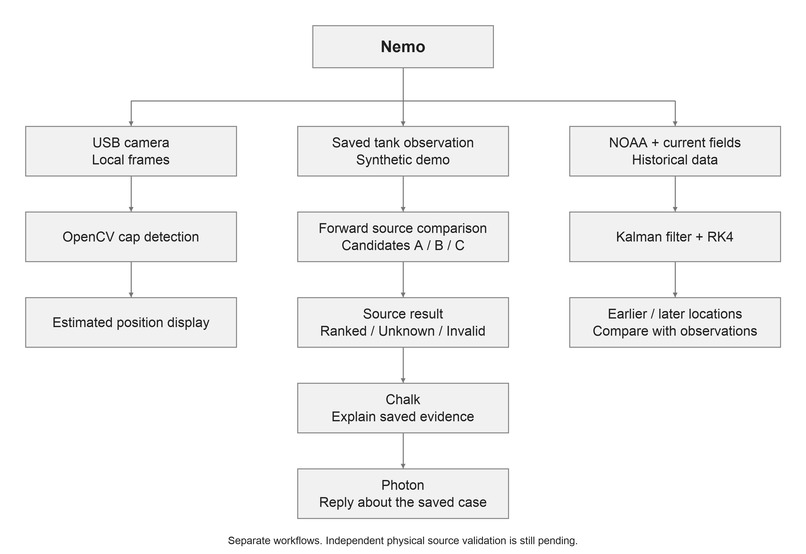
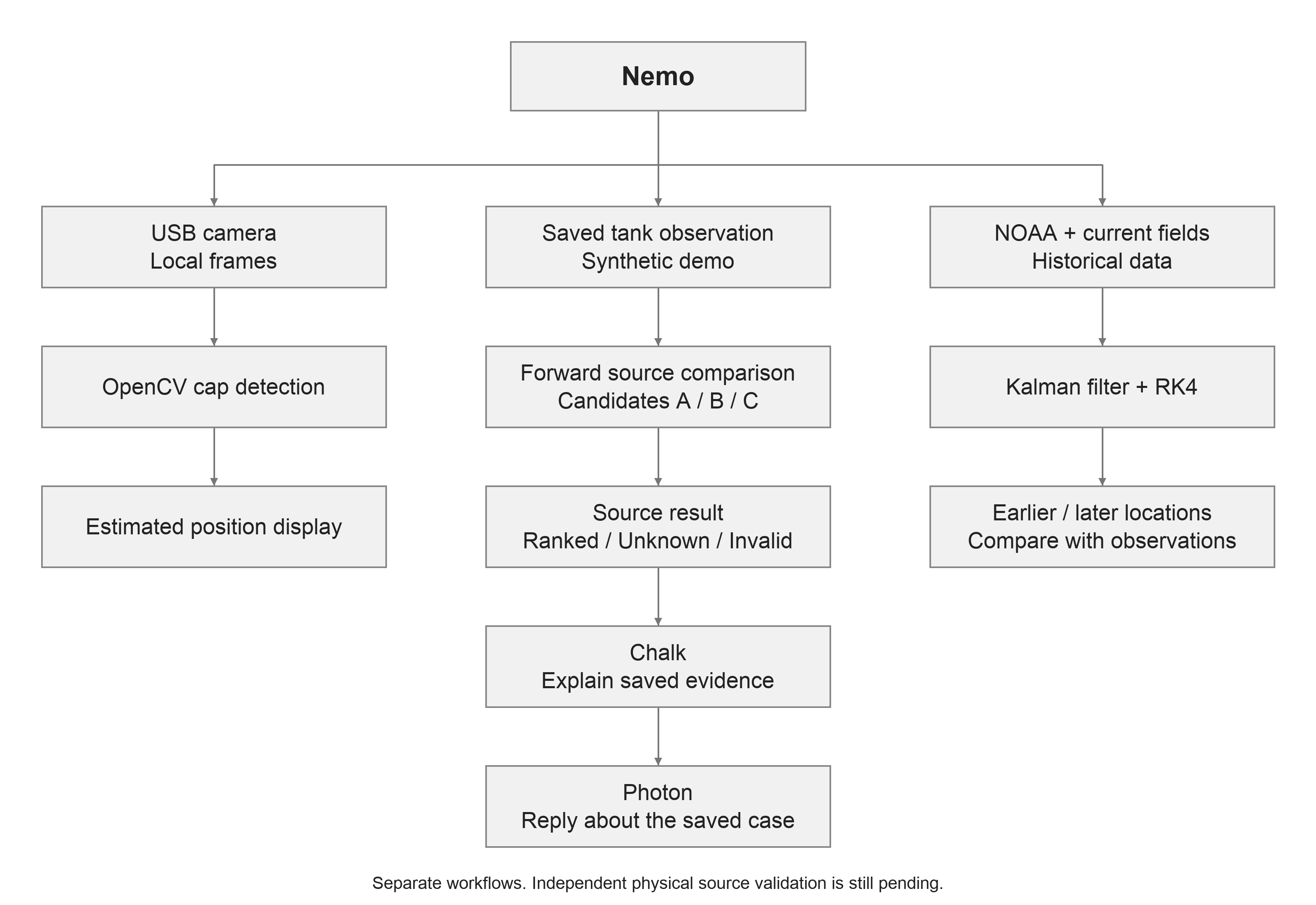
05. Nemo workflow: camera tracking, synthetic source comparison and historical ocean research.
-
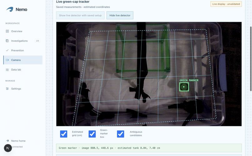
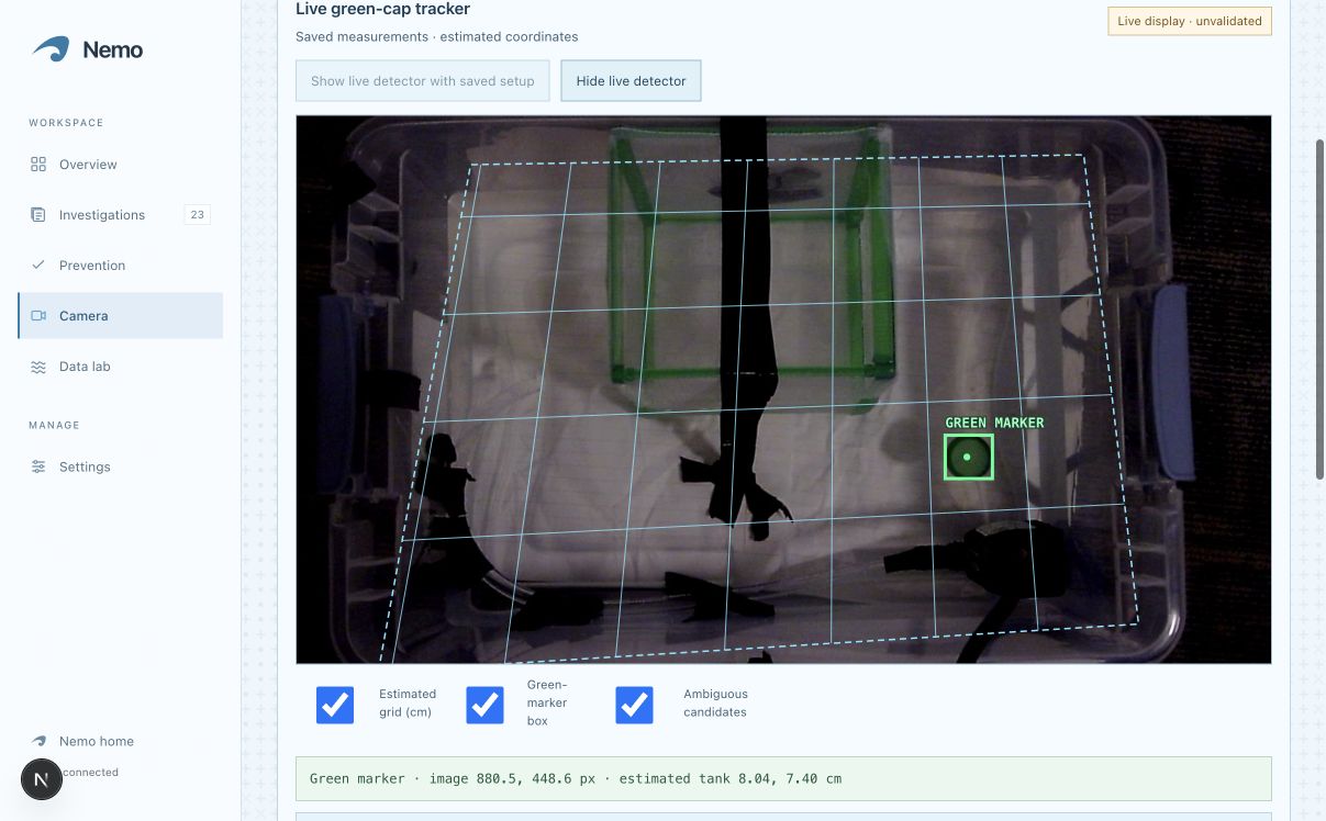
06. Live green-cap detection with the full tray and estimated grid. Frames stay local; centimetre accuracy is unvalidated.
-
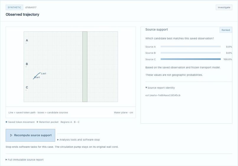
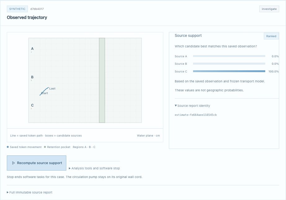
07. Synthetic source example: C best matches the saved trajectory. Support is conditional on the declared candidates.
-
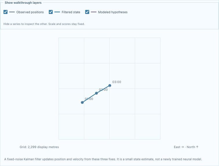
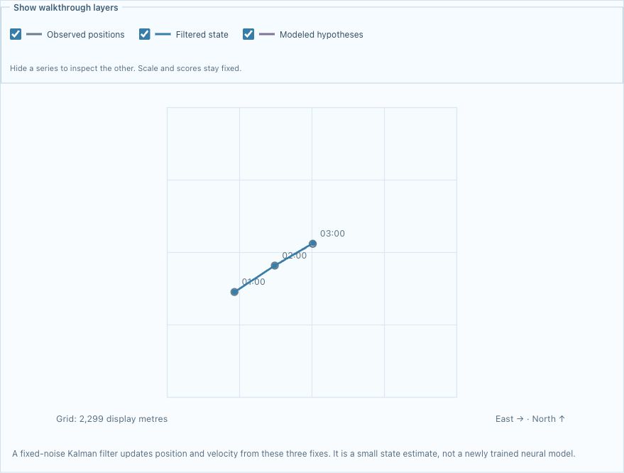
08. Kalman combines permitted observations with a motion estimate. Its assumed uncertainty is not measured buoy accuracy.
-
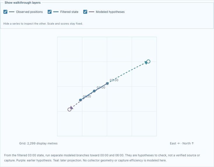
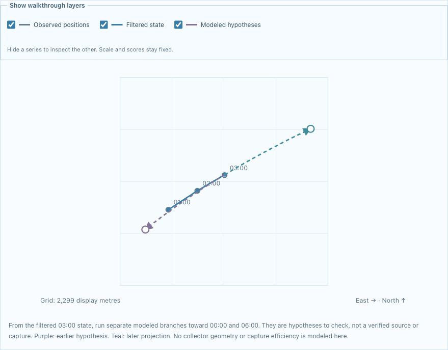
09. Purple explores earlier locations; teal projects later motion. These hypotheses do not establish a pollution origin.
-
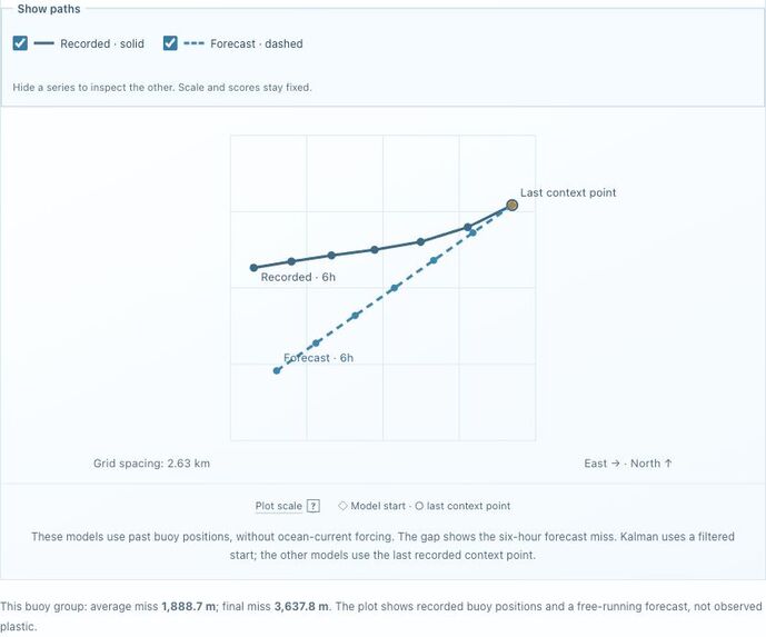
10. Recorded NOAA buoy motion versus a free-running six-hour forecast. The gap is prediction error.
-
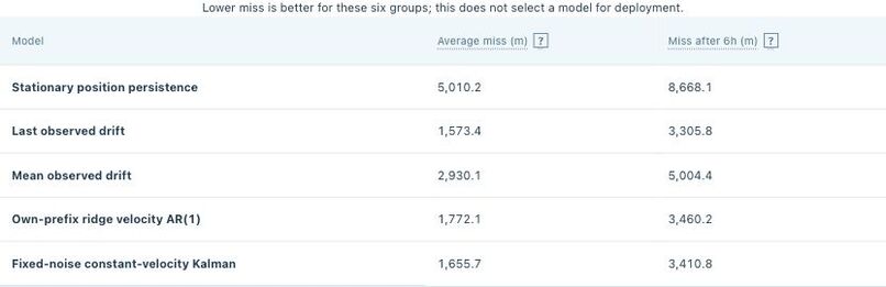
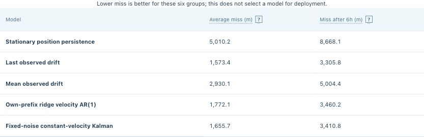
11. Five fixed models, six historical buoy groups. Last drift has the lowest average miss here; no automatic model promotion.
-
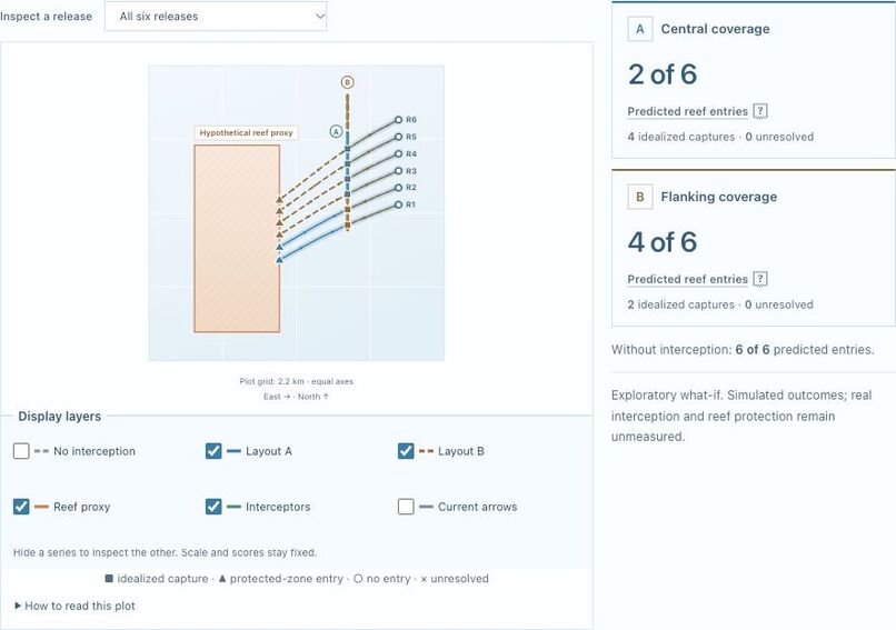
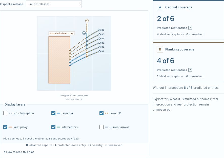
12. Changing currents: central layout predicts 2/6 entries, flanking 4/6 and no interception 6/6. Simulated outcomes.
-
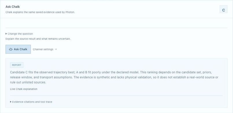
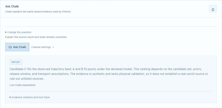
13. Live Chalk explains the saved source report. Python computes the numbers; citations anchor the explanation.
-
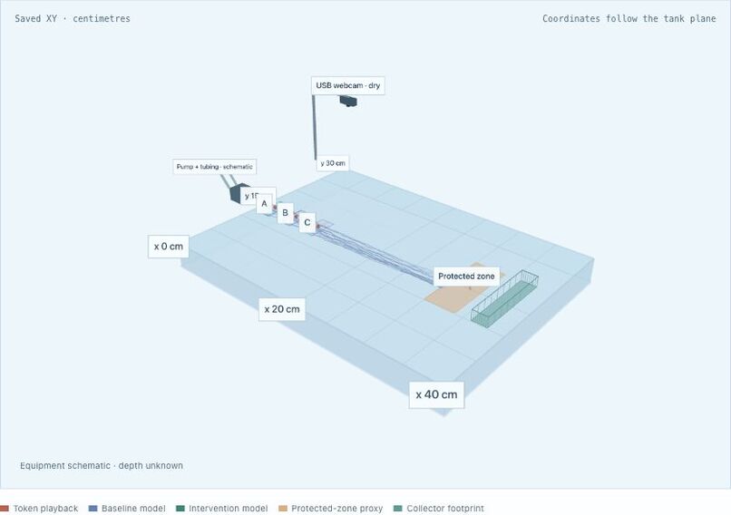
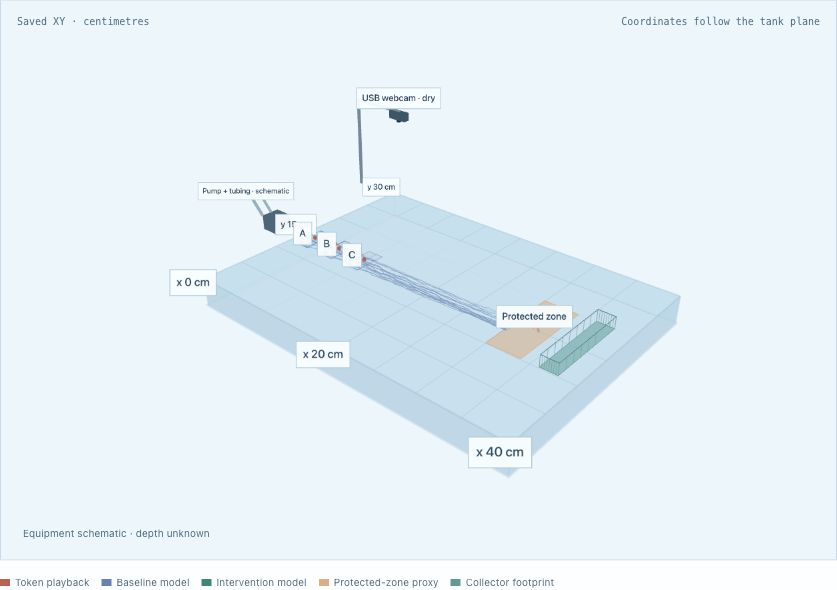
14. Nemo 3D rehearsal: complete 40 × 30 cm synthetic scene, saved paths, protected-zone proxy and collector.
-

15. Photon: a natural question and verified automatic reply about the saved synthetic source case.
Inspiration
When floating trash reaches a shoreline, we can see where it stopped. But where did it enter the water? And where could we collect the next piece before it reaches a vulnerable habitat?
Nemo connects those questions. Source tracing is our main purpose; prevention is the next decision. We began with an experiment we could see and understand: a green bottle cap representing floating trash, three possible entry regions, a webcam, a pump and a mesh collector.
Our goal is to help coastal teams investigate possible pollution pathways and choose collection plans worth testing. Today, Nemo is a working research prototype, not a validated worldwide pollution-source finder.
What it does
Nemo brings observation, modeling and explanation into one workspace, with three distinct evidence paths:
- Real camera observation: OpenCV finds a green cap in our tray. This verifies marker visibility, not source accuracy.
- Synthetic source investigation: saved simulated paths demonstrate how Nemo compares possible entry regions and handles uncertainty.
- Historical ocean research: real archived NOAA buoy positions test motion models and earlier/later position hypotheses.
These paths inform the same research goal without being presented as one completed physical experiment.
What are A, B and C?
They are candidate regions where an object could have entered the tank. Nemo simulates possible journeys from those regions and compares them with the saved observed path. In our synthetic example, C fits best under the declared assumptions. The support bars describe compatibility within those candidates, not a calibrated probability or proof of a polluter's identity.
The estimator can return Ranked, Unknown or Invalid. A cap first seen trapped at a collector may not reveal its earlier journey. Returning Unknown is useful: it tells the operator that another observation or a different experiment is needed.
Our physical prototype
Our rig uses a Logitech C270 USB webcam, a clear tray, a Pond Boss 80 GPH pump, about three feet of 3/8-inch-inside-diameter tubing, a mesh collection pocket and reusable green caps. Megana measured the inside waterline as 35.56 × 22.86 cm. A person operates the pump using its separate original power cord; Nemo does not control it electronically.
These hardware illustrations explain placement and tubing routes. Their arrows show intended circulation, not a measured flow field. The third illustrates an alternative without tubing.
The local detector uses color and shape checks to find our controlled green marker. It is not a general plastic classifier. Camera frames stay on the capture laptop. An estimated grid reuses saved geometry; unsupported alignment withholds centimetres. Independent alignment checks are required before positions can support measured trials. The pump's throughput rating is not the water velocity everywhere in the tray.
How the physics works
For tank source investigation, Nemo sends particles forward from each candidate region under declared drift, spreading and retention assumptions, then compares their histories with the observation. This tests possible journeys instead of assuming that one backward line reveals a unique origin.
The ocean walkthrough makes a different calculation visible. It starts with three permitted historical NOAA positions, connects them, and uses a causal Kalman filter to estimate position and velocity. The connected line is a visual estimate between fixes, not newly observed movement.

updated state = predicted state + weighted measurement correction
The filter balances model and measurement uncertainty. It does not read reserved comparison positions to improve its answer. Its noise assumptions are not independently measured buoy accuracy or settings transferable to our centimetre-scale tank.
The walkthrough's next rule is:
particle motion = modeled current(position, time) + fixed initial motion offset
The offset is filtered velocity minus modeled current at the final permitted observation, held fixed afterward. RK4 integrates that field forward and backward through the appropriate times. Purple explores earlier positions; teal projects later motion. Neither branch identifies the object's release time or proves a pollution source. Backward integration cannot undo mixing, beaching or capture.
Real data, including results that challenged us
We use archived NOAA Global Drifter Program positions, historical HYCOM currents, a saved PacIOOS ROMS current forecast and separate NOAA Coral Reef Watch heat-stress context. Buoys are not plastic. HYCOM's saved 15-metre depth limits its relevance to surface debris, while reef heat stress provides habitat context rather than source evidence.
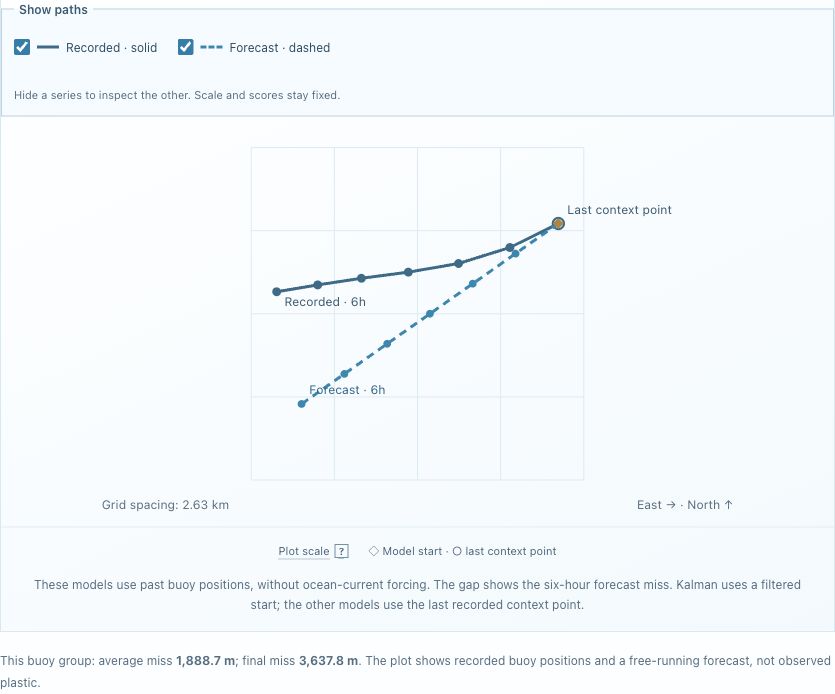
One frozen comparison evaluated five fixed models on six new-to-project historical buoy groups: 180 model-hour outcomes against 36 distinct later positions. Mean position error was about 1,573 m for last observed drift, 1,656 m for Kalman and 1,772 m for ridge velocity AR(1). The simple last-drift baseline performed best on this cohort. Reusing targets across methods does not create independent experiments.
A separate retrospective reverse-current test missed earlier positions by 8.70 km on average, versus 2.20 km for last-drift extrapolation on two already-viewed targets. We kept this unfavorable result. Reversing a forward model alone does not validate pollution-source inference, and a tiny numerical round-trip error does not prove the recovered past is correct.
From a source question to a prevention experiment
The ocean comparison applies equal-length interception layouts to the same six hypothetical releases under changing currents. It predicts six reef-proxy entries without interception, two with layout A and four with B. Capture is idealized, and the receiving-area proxy was chosen after viewing the forecast. The result suggests a scenario to test, not measured reef protection.
The Three.js tank scene renders saved geometry and representative paths. Users can orbit, switch layouts and scrub time while full-report counts stay fixed. Its stock 40 × 30 cm synthetic scene is separate from our 35.56 × 22.86 cm physical tray. Equipment and depth are schematic; this is a rehearsal, not a validated fluid simulation. The trial ledger distinguishes predictions, synthetic outcomes and reported physical trials, retaining unresolved or missing releases.
Chalk, Photon and Grok
Python computes the scientific results. Chalk helps explain them. A question is attached to the selected case. Our backend checks permissions and report identity, then exposes bounded evidence tools to a language model through Chalk Model Gateway. The returned explanation must satisfy its action contract and cite permitted evidence; stale or invalid output is rejected.
Here, Chalk explains why C fits the saved synthetic path and describes the candidate, release-window and transport assumptions. Citations and the tool trace connect its words to the report. A provider failure leaves the numerical evidence available and cannot upgrade Unknown to an accepted source.
Photon brings the same saved-case investigator into iMessage. We verified an actual delivered automatic reply to a natural source-evidence question. The authorized conversation is pinned to a saved case; it does not silently follow the live cap. A local worker handles messaging with durable inbox/outbox records and idempotent retries. Hosted Photon checks project authentication read-only.

Grok helped us challenge the implementation. We used it for physics research, model comparisons, causal filtering, RK4, reverse-source limitations and test design, with Cursor contributing to development. We checked suggestions against code, data and tests and retained reviews and corrections. Our Python backend executes the calculations.
Building, testing and learning
Python, FastAPI, Pydantic, OpenCV, NumPy, SciPy and SQLite support the services. Next.js, React and TypeScript provide the interface. GitHub Actions checks changes, and Render hosts the software demo; full webcam processing stays on the local companion.
Verification covered source states, evidence freshness, authentication, NOAA stages, trajectory toggles, frame/box identity, 3D playback, messaging retries and provider failure paths. Separate live checks obtained a Chalk explanation and a visible Photon reply. These software and integration checks do not establish physical prediction accuracy.
Our hardest practical challenge was getting usable evidence. Shadows, ripples, small camera shifts and cap retention affected recordings. We excluded unusable wet runs instead of treating trapped-cap jitter as water flow. No independently validated physical source or interception result has been established.
What's next
We will check current alignment, record separate flow-training and validation runs, freeze the method, and conduct blind known-source releases. The evaluator keeps the true source hidden until Nemo saves its answer. Correct, incorrect, Unknown, invalid and missing outcomes all remain visible. Interception predictions then need independent observed entry and mesh-retention outcomes.
Nemo's long-term purpose is practical: help teams investigate where pollution could enter the water and decide where collection equipment deserves a real test. Our prototype connects that decision to evidence people can inspect.


Log in or sign up for Devpost to join the conversation.