
Inspiration
We wanted to beat the commodities market. Our first instinct was gold — it felt like the "safe" choice.
Then we looked at what was actually happening. Gold had fallen 28% from its January high with an FOMC meeting days away. Oil was moving 6% in a single session on Iran headlines. Both were coinflips dressed up as analysis.
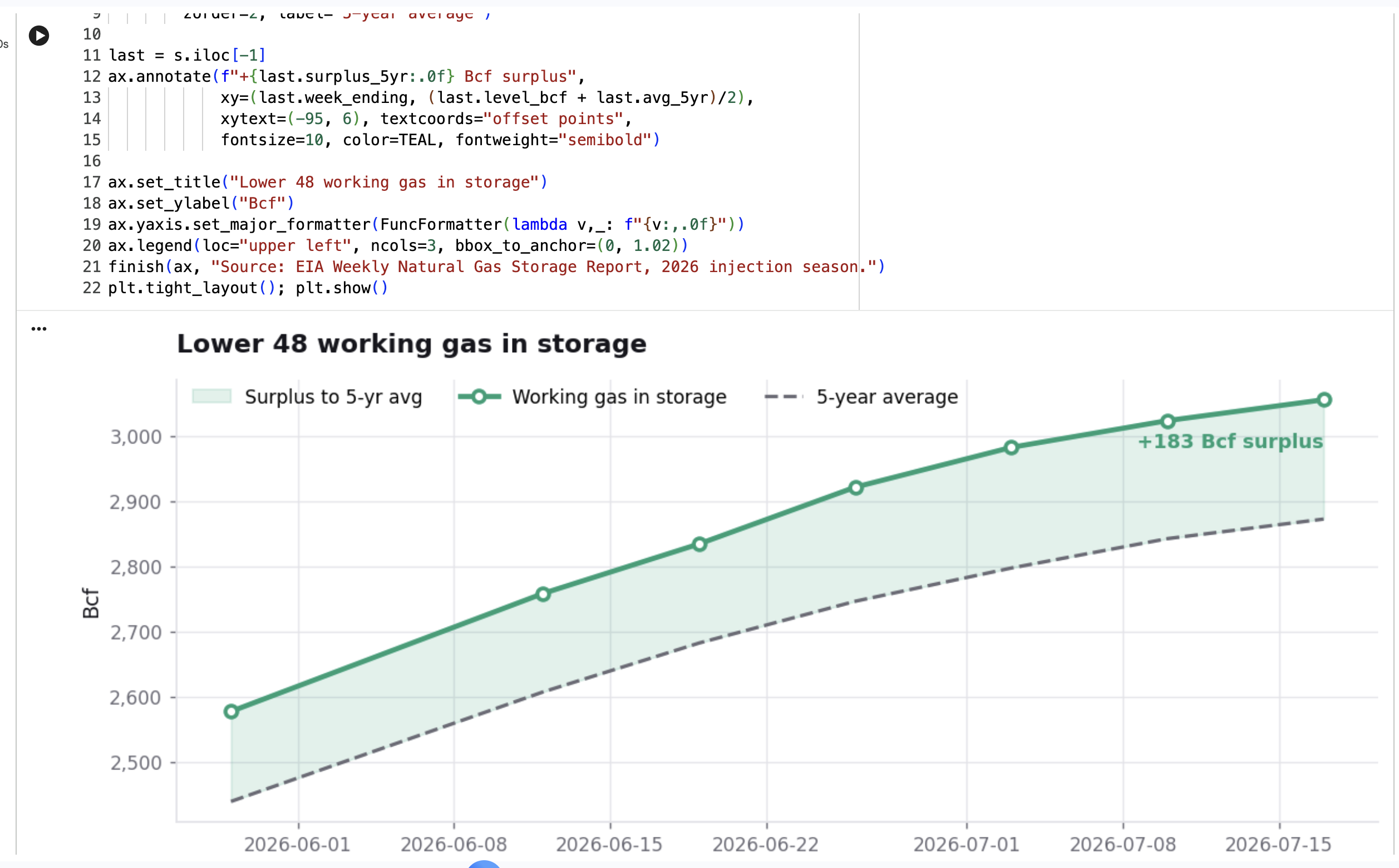
Natural gas was the one that stood out, for a reason that felt almost unfair: it's a physical market with a single balancing variable. Gold's price is a story about interest rates and sentiment. Gas is molecules going into and out of the ground, and the US government measures it every Thursday at 10:30 AM Eastern.
That gave us a thesis we could actually defend:
We are not predicting the price of natural gas. The market already has a forecast, and it is very good. We are predicting the market's error.
What it does
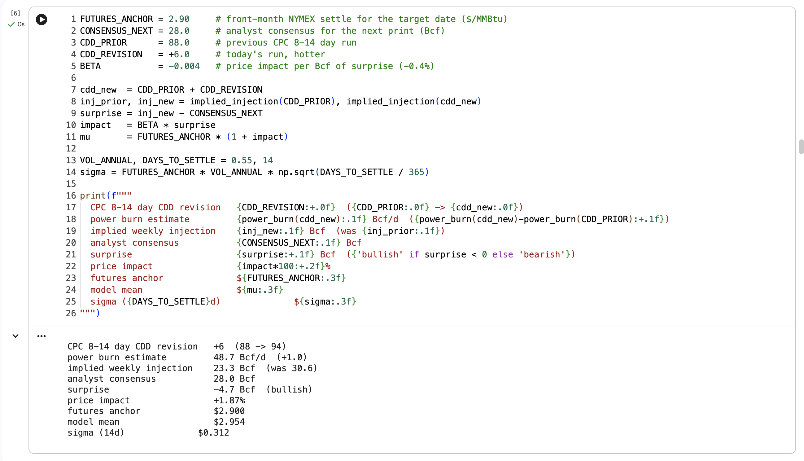
Our agent forecasts Kalshi threshold contracts — will Henry Hub settle above $K — by computing a causal chain rather than pattern-matching price history:
weather forecast revision
  → population-weighted cooling degree days
  → gas burned for electricity generation
  → weekly supply/demand balance
  → implied storage injection
  → surprise vs analyst consensus
  → price deviation from the futures anchor
  → P(settle > K)
Every arrow is a function we wrote. Nothing is a black box, and every prediction ships with the full chain so a human can audit it and disagree at any step.
How we built it
The balance model. Weekly storage injection is whatever supply is left after demand takes its share:
$$\text{injection} = 7 \times \left(P_{\text{dry}} - D_{\text{power}} - D_{\text{res}} - D_{\text{ind}} - D_{\text{LNG}} - D_{\text{exp}} - D_{\text{fuel}}\right)$$
In summer, power burn is the only term that moves meaningfully week to week — so the entire model collapses to one relationship:
$$D_{\text{power}} = \alpha + \beta \cdot \text{CDD}$$
We recovered $\alpha$ and $\beta$ by least squares against the real 2026 EIA prints.
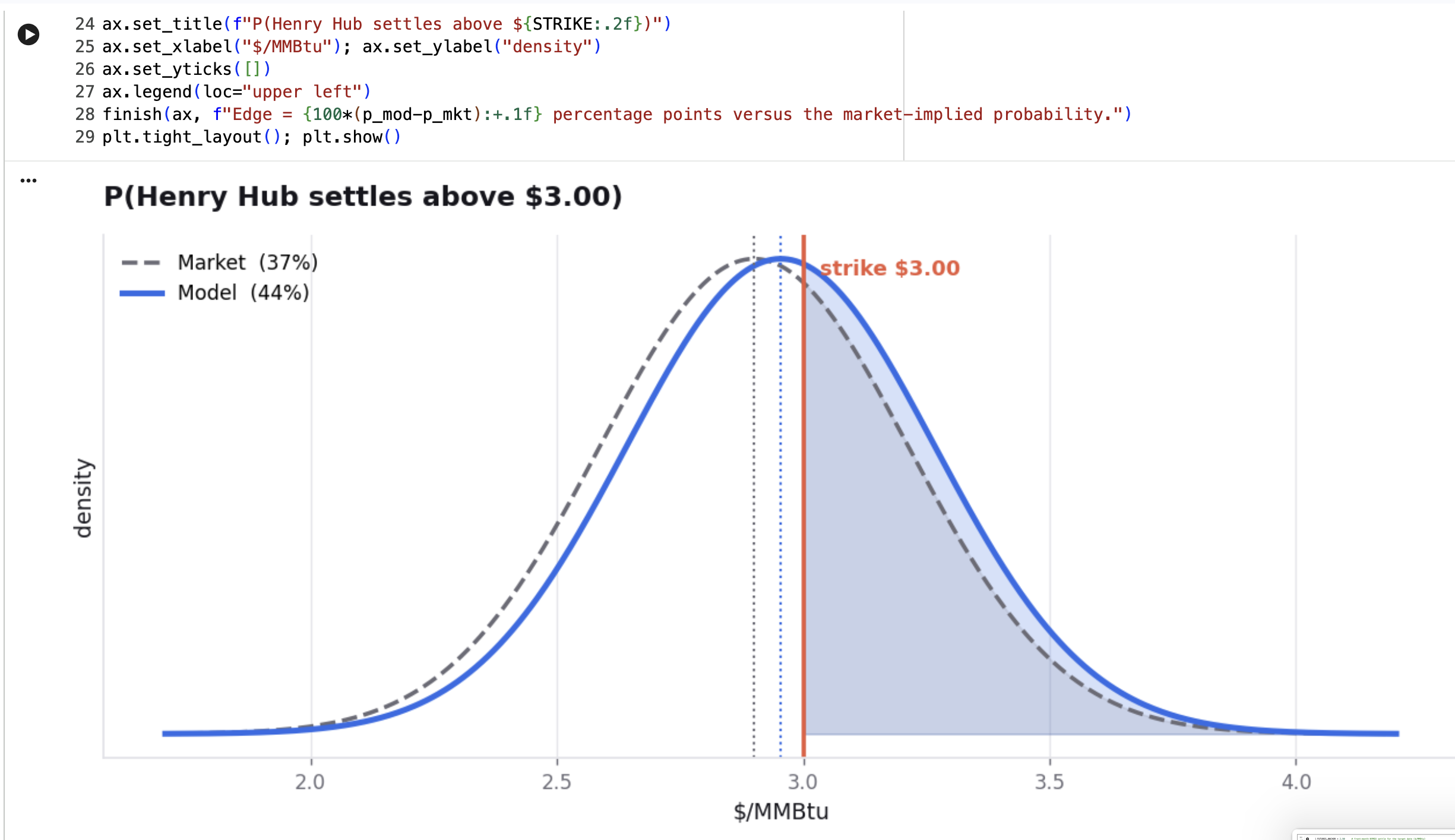
The Kalshi conversion. This is where our understanding changed most. A threshold contract needs a probability, not a price, which means you need a full distribution:
$$P(\text{settle} > K) = 1 - \Phi!\left(\frac{K - \mu}{\sigma}\right)$$
Two parameters. Everyone competes on $\mu$. Almost nobody competes on $\sigma$ — and $\sigma$ is where the edge lives, because you can have zero opinion on direction and still be right that the market has mispriced the width.
The LLM layer. The structural model has one fatal blind spot: it cannot see news. We added an analyst that reasons about mechanism rather than sentiment, with US gas market structure encoded in its system prompt. Critically, the LLM never outputs the probability — LLMs are bad at arithmetic and worse at calibration. It reasons about news and sets weights; the number stays numerical.
Stack: Python, NumPy, SciPy, Matplotlib, EIA API v2, NOAA CPC, Kalshi API, Fireworks for inference.
What we learned
Price responds to the surprise, not the level. The Thursday report covers a week that ended six days earlier. If markets were efficient about the past it shouldn't move prices at all — yet it moves them 2–5% in seconds. The reason: the EIA number is the only authoritative measurement of the supply-demand balance. It doesn't tell you about last week, it tells you how wrong your model of right now is — and that error is autocorrelated, so it gets extrapolated forward immediately.
Several relationships are backwards from intuition. These became the core of our LLM's system prompt:
- Gulf hurricanes are bearish for Henry Hub. Offshore production is down to ~1.6 Bcf/d, but an LNG terminal shutdown removes 2–3 Bcf/d of demand. The storm destroys demand, not supply.
- High oil prices are bearish for gas. Permian gas is an associated byproduct of oil drilling. More oil rigs means more gas nobody chose to produce.
- Global LNG disruptions are roughly neutral. When Iranian strikes damaged Ras Laffan (~20% of global LNG supply), European TTF jumped 32% overnight — and Henry Hub barely moved, because the US is supply-long and export-constrained.
That last one became our best demo. A sentiment classifier reads "LNG supply disruption" and says bullish. Our LLM correctly called it neutral and explained the offsetting mechanisms.
Consensus is not a single number. For the July 16 print, one desk called +41 Bcf a bearish surprise against a +36 consensus. Another called the identical number roughly in line against a +39 survey with a 38–45 range. Whichever series you benchmark against is a modeling choice you have to declare.
Challenges we ran into
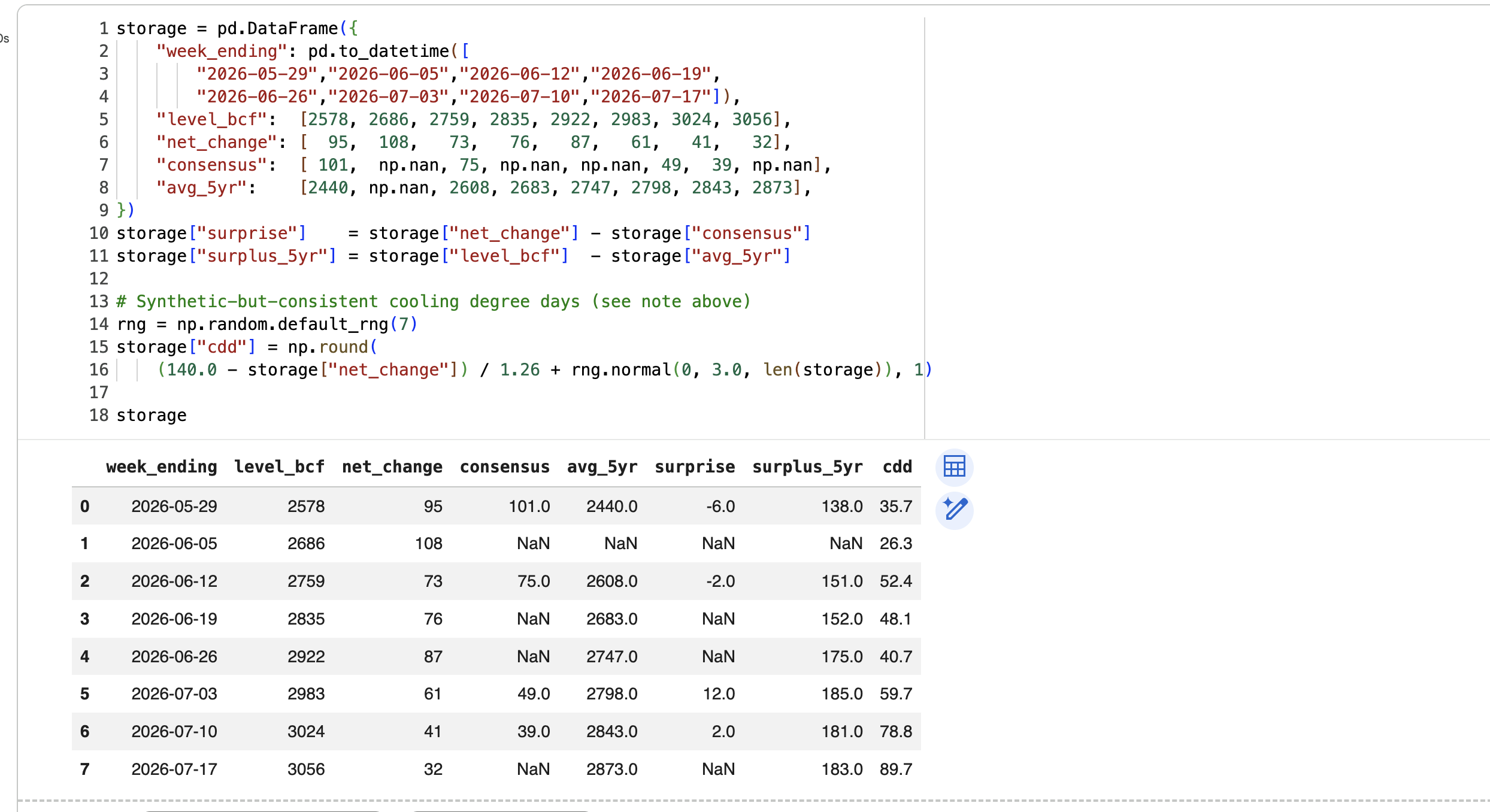
Look-ahead bias, which nearly got us. The Thursday report covers the week ending the previous Friday. A naive date join leaks six days of future information into every row. The backtest looks spectacular; the live model is worthless. We rebuilt every feature with a known_at timestamp and an as-of join. The same trap applies to weather — training on realized degree days instead of the forecast as issued builds a model that requires a time machine.
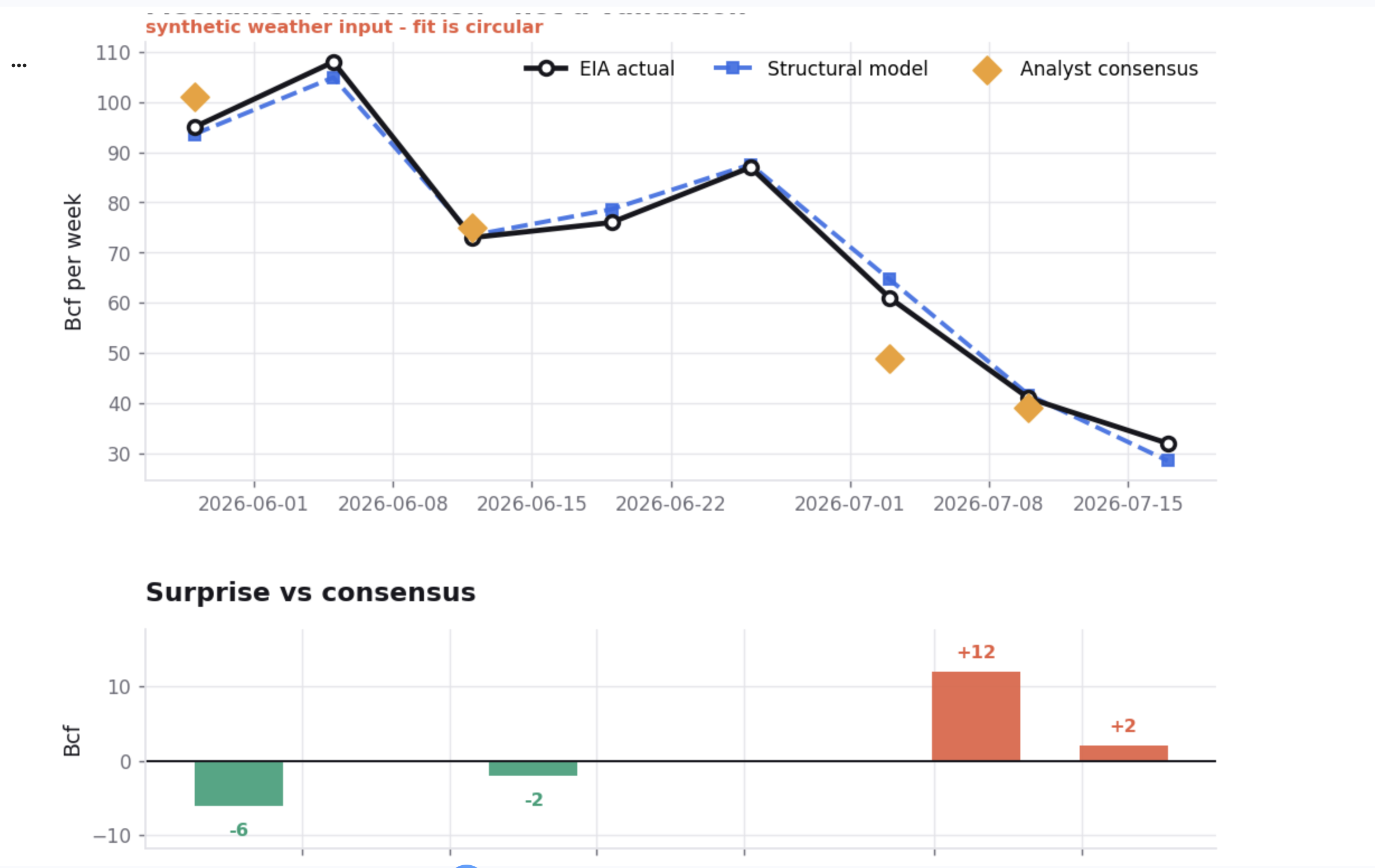
We caught ourselves reporting a meaningless result. Without a live NOAA feed, we back-solved a degree day series from the storage prints. Then we fit a linear model of injections on degree days and got a 2.0 Bcf error — better than professional analysts.
It was completely circular. We had derived the inputs from the outputs, so the fit recovered a relationship we had inserted by construction. It proved nothing except that we could invert a linear equation.
We relabeled the chart "mechanism illustration — not a validation," removed the accuracy claim, and put a warning banner at the top of the notebook. This is the thing we're most glad we caught, and we'd rather present an honest unvalidated model than a fake validated one.
The random walk is a brutal baseline. Most published commodity forecasting models fail to beat it once look-ahead bias is removed. Accepting this early changed what we built: instead of chasing a magic predictor, we built the evaluation harness first — Brier skill score against the market, calibration curves, PIT histograms — so that if we ever do find edge, we'll be able to believe it.
What's next
- Real NOAA CPC degree days, replacing the synthetic series. Our error will get worse, and that number will finally mean something.
- Validation at scale — 50+ resolved contracts with a Brier skill score and a confidence interval.
- Variance modeling. Whether an EIA report falls inside a contract window is a binary, knowable fact, and contracts spanning one should price visibly more variance. When they don't, that's a trade — and it doesn't require any view on direction.
- Fat tails. Gas returns are right-skewed; the normal distribution systematically underprices the upside. That skew is currently compressed by high storage but will matter enormously in winter.
- A meta-agent that repairs the model. Because every link in our chain has its own observable ground truth, a failed prediction yields per-link error attribution rather than one scalar loss. That's an automatically labeled failure dataset — the substrate for an agent that diagnoses which component drifted and fixes it.
Honest assessment
We have not validated this model. Our weather inputs are synthetic and our fit statistic is circular.
What we built is the architecture — a causal chain that is auditable at every step, a correct treatment of threshold contracts as distributions rather than point forecasts, an LLM layer that argues with us instead of agreeing with us, and an evaluation harness rigorous enough to tell us when we're wrong.
We think that's the right foundation. The edge comes next.

Log in or sign up for Devpost to join the conversation.