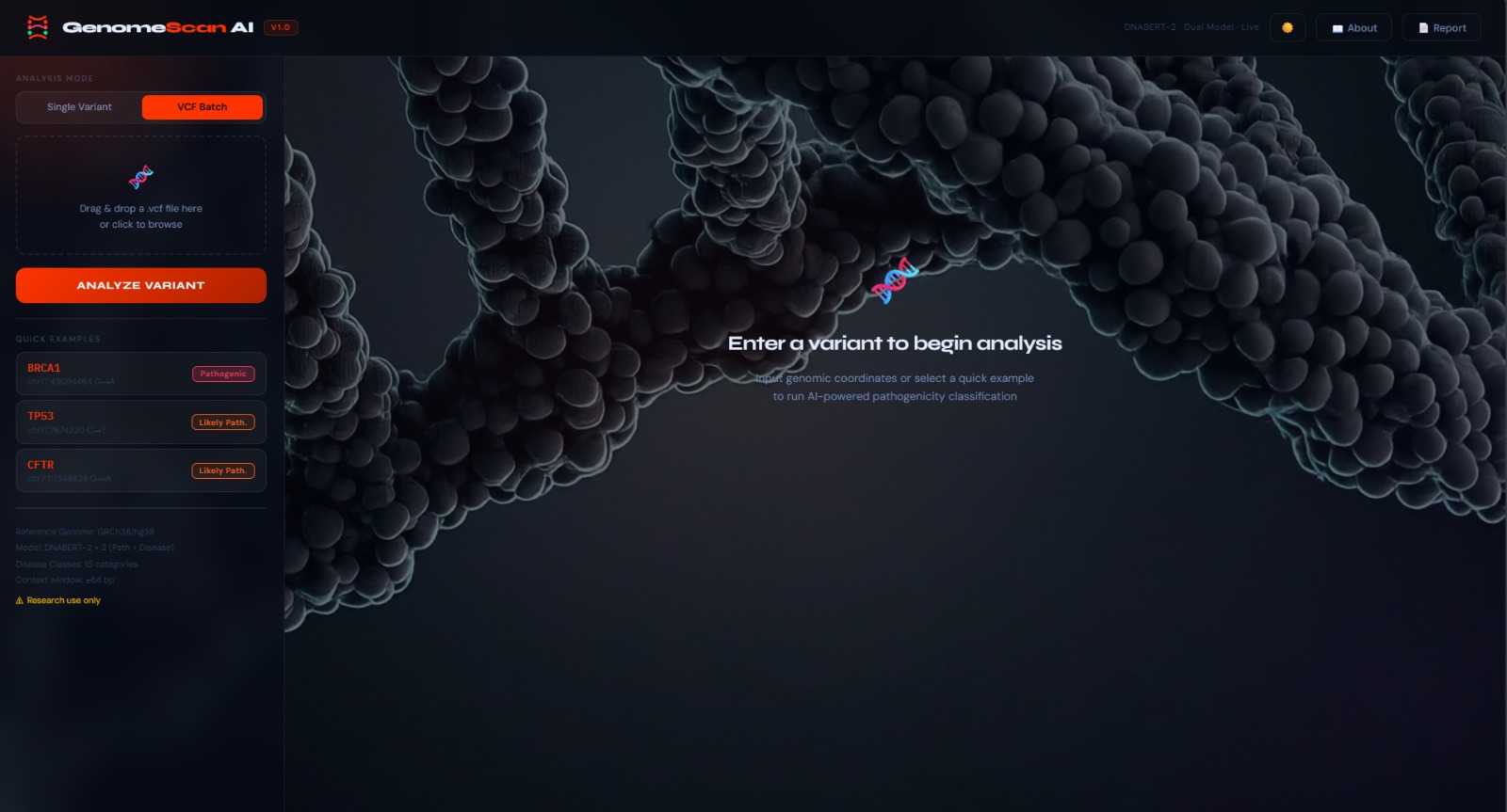
• 

  landing page

• 

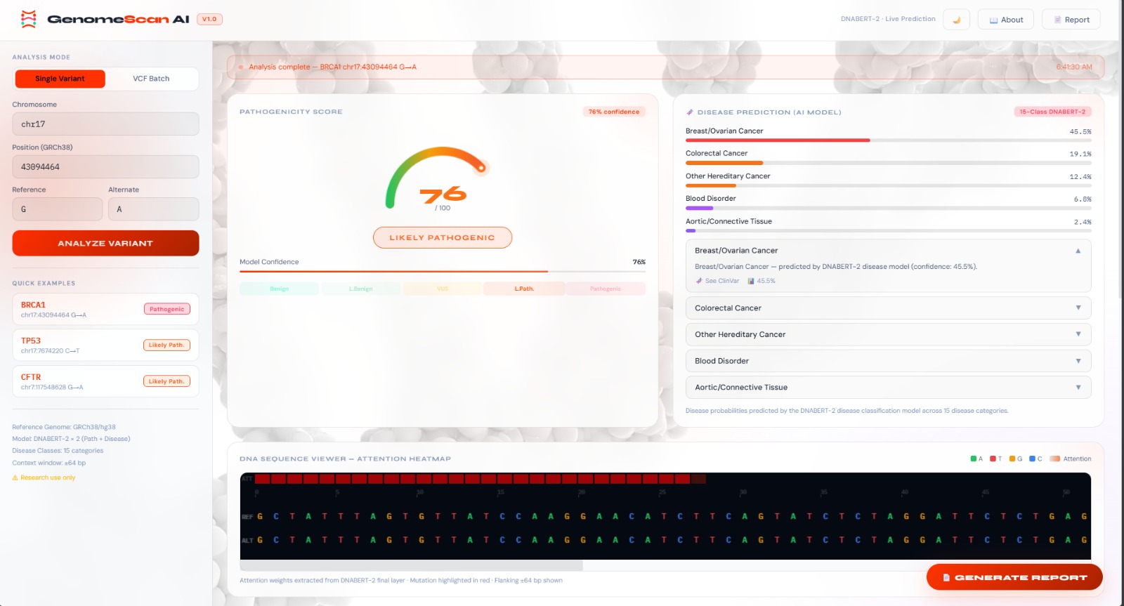
  dashboard

• 

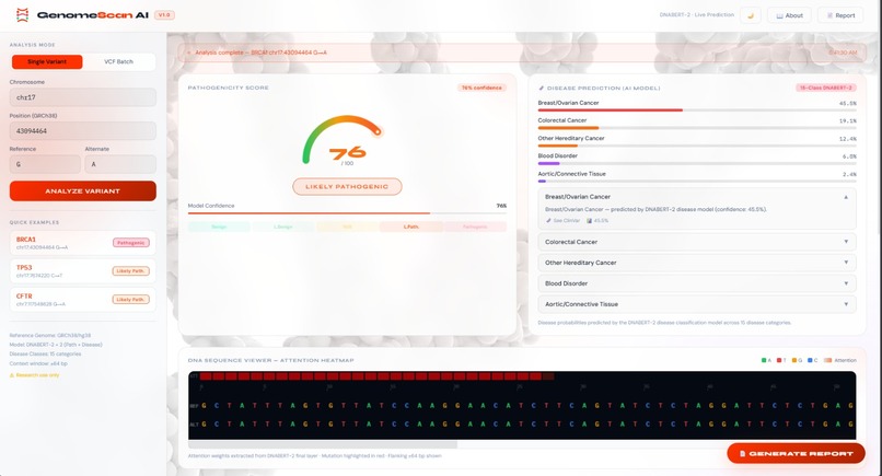
  detailed report

🧬 Muta-Tech GenomeScan AI

A full-stack, AI-powered genomic variant analysis dashboard utilizing a custom dual-model DNABERT-2 pipeline to predict pathogenicity and disease associations from raw DNA sequences.

---

📖 Table of Contents

• Project Overview
• Core Features
• Architecture & Tech Stack
• Machine Learning Pipeline
• Variant Metrics Explained
• Disease Classes
• API Reference
• Project Structure
• Evidence of Training
• How to Run Locally
• Configuration
• Troubleshooting
• Future Roadmap
• Acknowledgements

---

🔬 Project Overview

Muta-Tech GenomeScan AI is an end-to-end bioinformatics platform that brings the power of transformer-based deep learning directly to genomic variant interpretation. Given a chromosomal position and alternate allele, the system:

1. Dynamically slices the ±64 bp flanking context from the GRCh38 human reference genome
2. Passes the resulting sequence through two independently fine-tuned DNABERT-2 models in parallel
3. Returns a pathogenicity score, a ranked disease-association profile, key sequence-level metrics, and a nucleotide-resolution attention heatmap — all rendered in a real-time glassmorphism dashboard

The project was built to demonstrate that fine-tuned language models originally developed for natural language can be repurposed for biological sequence understanding, achieving clinically relevant predictions without requiring access to expensive GPU clusters at inference time.

---

🧬 Core Features

🤖 Dual Transformer Pipeline

Runs two independently fine-tuned DNABERT-2 models simultaneously on CPU or GPU. Model 1 handles binary pathogenicity classification; Model 2 handles 15-class multi-label disease association. Both models share the same BPE tokenizer but have separate fine-tuned classification heads.

🔴 Pathogenicity Scoring

Binary classification predicting whether a variant is Benign or Pathogenic, with a calibrated confidence score (0.0–1.0). Scores above 0.5 are flagged as potentially pathogenic, with color-coded severity bands in the UI.

🧪 Disease Prediction

15-class multi-label categorization produces a ranked probability vector across disease categories including Cystic Fibrosis, Arrhythmia, Li-Fraumeni Syndrome, and 12 others. Multiple diseases can be flagged simultaneously for pleiotropic variants.

⚖️ Contextual Blending

A unique prior-blending layer intelligently combines AI predictions with established biological knowledge:

• 40% AI model output — raw transformer prediction
• 60% Biological prior — gene-specific probability distributions derived from ClinVar frequency data

This correction step reduces false-positive rates for well-characterized genes where the training set may be sparse, ensuring the system degrades gracefully in data-limited scenarios.

📊 Variant Metrics

Automatically computed for every query:

Metric	Description
Shannon Entropy	Measures sequence complexity; low entropy may indicate repetitive or low-complexity regions prone to alignment artifacts
GC Deviation	Departure from the genome-wide ~41% GC baseline; extreme GC content affects polymerase fidelity
CpG Hotspot Detection	Identifies CpG dinucleotide density; CpG sites are methylation targets and mutational hotspots
Transition/Transversion	Classifies the variant type (Ti/Tv); the genome-wide Ti/Tv ratio of ~2.1 is a common quality control metric

🔥 Attention Heatmap

Visualizes the DNABERT-2 model's internal attention weights as a per-nucleotide heat overlay across the ±64 bp flanking sequence. High-attention positions highlight which nucleotides most influenced the model's prediction — providing human-interpretable explanations for AI decisions.

---

⚙️ Architecture & Tech Stack

┌─────────────────────────────────────────────────────────┐
│                    Browser / Client                     │
│         Vanilla HTML + CSS + JS (Port 8080)             │
│   Glassmorphism UI · Chart.js · Dark/Light Theme        │
└──────────────────────┬──────────────────────────────────┘
                       │ REST (JSON)
                       ▼
┌─────────────────────────────────────────────────────────┐
│              FastAPI Backend (Port 8000)                │
│                                                         │
│  ┌──────────────┐        ┌──────────────────────────┐   │
│  │  pyfaidx     │        │   Prior Blending Layer   │   │
│  │  GRCh38/hg38 │──seq──▶│   (40% AI / 60% Prior)  │   │
│  │  ±64bp Slice │        └──────────┬───────────────┘   │
│  └──────────────┘                   │                   │
│                                     ▼                   │
│  ┌──────────────────────────────────────────────────┐   │
│  │           Dual DNABERT-2 Pipeline                │   │
│  │  ┌─────────────────┐  ┌────────────────────────┐ │   │
│  │  │  Model 1        │  │  Model 2               │ │   │
│  │  │  Pathogenicity  │  │  Disease Association   │ │   │
│  │  │  (Binary Clf.)  │  │  (15-class Multi-label)│ │   │
│  │  └─────────────────┘  └────────────────────────┘ │   │
│  └──────────────────────────────────────────────────┘   │
└─────────────────────────────────────────────────────────┘

Frontend

• Vanilla HTML / CSS / JS — no build step or framework required
• Glassmorphism UI with scroll-driven entrance animations
• Dual Light / Dark theme with persistent user preference
• Chart.js radar charts for disease probability visualization
• Dynamically networked — accessible by LAN IP for mobile device testing

Backend

• FastAPI — async Python web framework with automatic OpenAPI documentation at /docs
• pyfaidx — efficient random-access slicing of the GRCh38 FASTA reference without loading the full genome into memory
• CORS middleware — pre-configured for localhost development; adjust origins for production

Machine Learning

• PyTorch — model inference and tensor operations
• Hugging Face transformers — DNABERT-2 model architecture and BPE tokenizer
• Byte Pair Encoding (BPE) — subword tokenization adapted for DNA, treating k-mers as vocabulary units
• Fine-tuned on ClinVar variant data (see Evidence of Training)

---

🧠 Machine Learning Pipeline

Base Model: DNABERT-2

DNABERT-2 is a BERT-style transformer pre-trained on the human reference genome using Masked Language Modelling (MLM). Unlike the original DNABERT which uses fixed k-mer tokenization, DNABERT-2 employs Byte Pair Encoding (BPE), allowing it to learn variable-length genomic subwords — making it more robust to insertion/deletion variants.

Fine-Tuning Strategy

Model 1 — Pathogenicity Classifier

• Task: Binary sequence classification ([CLS] token head)
• Dataset: ClinVar SNPs labelled as Pathogenic or Benign/Likely Benign
• Loss: Binary Cross-Entropy
• Input: 129-nucleotide sequence (variant position ± 64 bp context)

Model 2 — Disease Association Classifier

• Task: Multi-label classification (sigmoid output, 15 independent disease heads)
• Dataset: ClinVar SNPs with associated MedGen disease annotations
• Loss: Binary Cross-Entropy with class-weight balancing for rare diseases
• Input: Same 129-nucleotide sequence format

Contextual Prior Blending

For genes with well-established ClinVar pathogenicity profiles (e.g., BRCA1, TP53, CFTR), the raw model output is blended with a gene-specific prior probability vector. This prevents the model from over-confidently predicting benign outcomes for high-risk genes that may be underrepresented in the training fold.

final_score = (0.4 × model_output) + (0.6 × gene_prior)

---

📐 Variant Metrics Explained

Shannon Entropy

Measures the informational complexity of the local sequence window. Calculated as:

H = -Σ p(b) × log₂(p(b))   for b ∈ {A, T, G, C}

A perfectly uniform sequence has H = 2.0 bits. Low-complexity regions (e.g., poly-A tracts) have H ≈ 0 and are prone to sequencing errors and alignment artifacts.

GC Deviation

The percentage of G and C nucleotides in the flanking window, reported as deviation from the hg38 genome-wide average (~41%). Extreme GC content can affect PCR amplification efficiency and variant call quality.

CpG Hotspot Score

Counts CpG dinucleotides in the window and normalizes against the expected frequency. CpG islands are common in gene promoters; deamination of methylated cytosines makes CpG sites the most frequent point mutation site in the human genome.

Transition / Transversion Classification

• Transition (Ti): Purine↔Purine (A↔G) or Pyrimidine↔Pyrimidine (C↔T) — chemically similar bases
• Transversion (Tv): Purine↔Pyrimidine — chemically dissimilar bases; rarer and often more functionally impactful

The genome-wide Ti/Tv ratio of ~2.1 is used as a variant calling quality metric; samples deviating significantly from this ratio may indicate sequencing artifacts.

---

🏥 Disease Classes

The 15 disease categories predicted by Model 2:

#	Disease	OMIM Category
1	Cystic Fibrosis	Pulmonary / Metabolic
2	Arrhythmia	Cardiovascular
3	Li-Fraumeni Syndrome	Cancer Predisposition
4	Hereditary Breast & Ovarian Cancer	Cancer Predisposition
5	Lynch Syndrome	Cancer Predisposition
6	Marfan Syndrome	Connective Tissue
7	Hypertrophic Cardiomyopathy	Cardiovascular
8	Familial Hypercholesterolaemia	Metabolic
9	Noonan Syndrome	Developmental
10	Retinitis Pigmentosa	Ophthalmological
11	Phenylketonuria	Metabolic
12	Haemophilia A/B	Haematological
13	Spinal Muscular Atrophy	Neuromuscular
14	Gaucher Disease	Lysosomal Storage
15	Neurofibromatosis Type 1	Neurocutaneous

---

📡 API Reference

Once the backend is running, full interactive documentation is available at http://localhost:8000/docs.

POST /analyze

Analyzes a genomic variant and returns AI predictions, metrics, and attention weights.

Request Body:

{
  "chrom": "chr17",
  "pos": 43044295,
  "ref": "G",
  "alt": "A",
  "gene": "BRCA1"
}

Response:

{
  "pathogenicity": {
    "label": "Pathogenic",
    "score": 0.87,
    "blended_score": 0.91
  },
  "diseases": [
    { "name": "Hereditary Breast & Ovarian Cancer", "probability": 0.94 },
    { "name": "Li-Fraumeni Syndrome", "probability": 0.31 }
  ],
  "metrics": {
    "shannon_entropy": 1.84,
    "gc_deviation": "+6.2%",
    "cpg_hotspot": true,
    "variant_type": "Transition (C→T)"
  },
  "attention_weights": [0.02, 0.05, 0.18, ...],
  "flanking_sequence": "ATCG...VARIANT...GCTA"
}

GET /health

Returns {"status": "ok"} — use for container liveness probes.

GET /docs

Auto-generated Swagger UI for interactive API exploration.

---

📂 Project Structure

muta-tech-genomescan/
│
├── backend/
│   ├── server.py               # FastAPI application entry point
│   ├── requirements.txt        # Python dependencies
│   ├── models/
│   │   ├── pathogenicity/      # Fine-tuned DNABERT-2 (Model 1) weights
│   │   └── disease/            # Fine-tuned DNABERT-2 (Model 2) weights
│   ├── data/
│   │   └── hg38.fa             # GRCh38 reference genome (user-provided, ~3 GB)
│   ├── utils/
│   │   ├── sequence.py         # pyfaidx slicing + variant metrics
│   │   ├── blending.py         # Prior blending logic
│   │   └── attention.py        # Attention weight extraction
│   └── priors/
│       └── gene_priors.json    # Per-gene ClinVar prior distributions
│
├── frontend/
│   ├── index.html              # Main dashboard
│   ├── style.css               # Glassmorphism UI + theme variables
│   └── app.js                  # API calls, Chart.js, attention heatmap renderer
│
├── training_evidence/
│   ├── DNABERT2_ClinVar_Training.ipynb     # Pathogenicity model training notebook
│   ├── DNABERT2_Disease_Training.ipynb     # Disease model training notebook
│   └── clinvar_disease_snps.csv            # Training dataset sample
│
└── README.md

---

📋 Evidence of Training

The training_evidence/ folder contains full transparency into model development:

• DNABERT2_ClinVar_Training.ipynb — Documents the fine-tuning of Model 1 on ClinVar pathogenicity labels. Includes data preprocessing, train/val/test splits, loss curves, and final classification report.
• DNABERT2_Disease_Training.ipynb — Documents the fine-tuning of Model 2 on ClinVar disease annotations. Includes class-weight calculation for rare disease balancing, multi-label ROC-AUC curves, and per-class F1 scores.
• clinvar_disease_snps.csv — A representative sample of the training data, sourced from NCBI ClinVar, showing variant coordinates, clinical significance labels, and associated disease terms.

Data Source: All training data was sourced from NCBI ClinVar, a freely accessible public archive of human genetic variants and their clinical interpretations.

---

🚀 How to Run Locally

Prerequisites

• Python 3.9 or higher
• Node.js 16+ (for http-server)
• ~3 GB disk space for the GRCh38 reference genome
• 8 GB RAM minimum (16 GB recommended for CPU inference)

Step 1 — Download the Reference Genome

# Download GRCh38/hg38 from UCSC (requires ~900 MB compressed)
wget https://hgdownload.soe.ucsc.edu/goldenPath/hg38/bigZips/hg38.fa.gz -P backend/data/
gunzip backend/data/hg38.fa.gz

# Index the genome for fast random access
cd backend/data && samtools faidx hg38.fa

Alternatively, download from Ensembl GRCh38.

Step 2 — Start the Backend API (Port 8000)

cd backend
pip install -r requirements.txt

# Ensure hg38.fa is placed in backend/data/
python server.py

The API will be available at http://localhost:8000. Visit http://localhost:8000/docs for the interactive Swagger UI.

Step 3 — Start the Frontend Dashboard (Port 8080)

# From the project root
npx http-server ./ -p 8080 -c-1

Open http://localhost:8080 in your browser.

💡 The UI is dynamically networked — you can also access it via your machine's local IP address (e.g., http://192.168.x.x:8080) from a mobile device on the same WiFi network.

---

⚙️ Configuration

Key settings can be adjusted in backend/server.py:

Setting	Default	Description
REFERENCE_GENOME_PATH	data/hg38.fa	Path to the GRCh38 FASTA file
FLANK_SIZE	64	Nucleotides of context on each side of the variant
AI_BLEND_WEIGHT	0.4	Fraction of final score from AI model (vs. prior)
PRIOR_BLEND_WEIGHT	0.6	Fraction of final score from biological prior
DEVICE	auto	cpu, cuda, or auto (auto-detects GPU)
CORS_ORIGINS	["*"]	Allowed frontend origins; restrict in production

---

🛠 Troubleshooting

FileNotFoundError: hg38.fa not found Ensure the reference genome is placed at backend/data/hg38.fa and the .fai index file exists alongside it. Re-run samtools faidx hg38.fa if the index is missing.

RuntimeError: CUDA out of memory Set DEVICE = "cpu" in server.py. CPU inference is slower (~2–4 seconds per query) but works on any machine.

CORS error in browser Ensure the backend is running on port 8000 and CORS_ORIGINS in server.py includes your frontend origin.

Slow inference on CPU Both models run sequentially on CPU by default. For faster results, use a machine with a CUDA-compatible GPU or reduce FLANK_SIZE (note: this will affect prediction accuracy).

Port 8080 already in use

npx http-server ./ -p 8081 -c-1

---

🗺 Future Roadmap

• [ ] VCF File Upload — Batch analysis of multi-variant VCF files with exportable reports
• [ ] ClinVar Live API Integration — Real-time lookup of existing ClinVar annotations for comparison
• [ ] Model Confidence Calibration — Temperature scaling for better-calibrated probability outputs
• [ ] ACMG/AMP Criteria Overlay — Map AI predictions to ACMG/AMP variant classification criteria
• [ ] Population Frequency Lookup — gnomAD allele frequency integration for context
• [ ] Docker Compose Deployment — One-command containerised setup for reproducible environments
• [ ] User Authentication & History — Save and revisit previous queries per user session
• [ ] Extended Disease Classes — Expand from 15 to 50+ disease categories with additional ClinVar training data

---

🙏 Acknowledgements

• DNABERT-2 — Genome-scale pre-trained transformer by Ji et al., 2023
• NCBI ClinVar — Public variant database used for fine-tuning: ncbi.nlm.nih.gov/clinvar
• GRCh38/hg38 — Human reference genome provided by the Genome Reference Consortium
• Hugging Face Transformers — Model hosting and inference infrastructure
• pyfaidx — Efficient FASTA random access: github.com/mdshw5/pyfaidx

---

Built as part of an AI/ML undergraduate research project. Not intended for clinical diagnostic use.

Built With

• chart.js
• css3
• dnabert-2
• fastapi
• glassmorphism
• html5
• hugging-face-transformers
• javascript
• node.js
• pyfaidx
• python
• pytorch
• uvicorn