Inspiration
Is a drop of pond water, a culture or a sample alive and swimming? Answering that usually takes a microscope, a trained eye, and a lot of trust in whoever is looking. Phones already have good cameras and capable GPUs, so we wanted to see whether two phones could answer the question quantitatively.
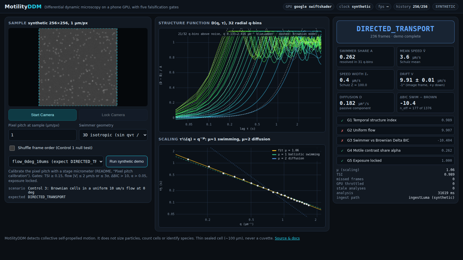
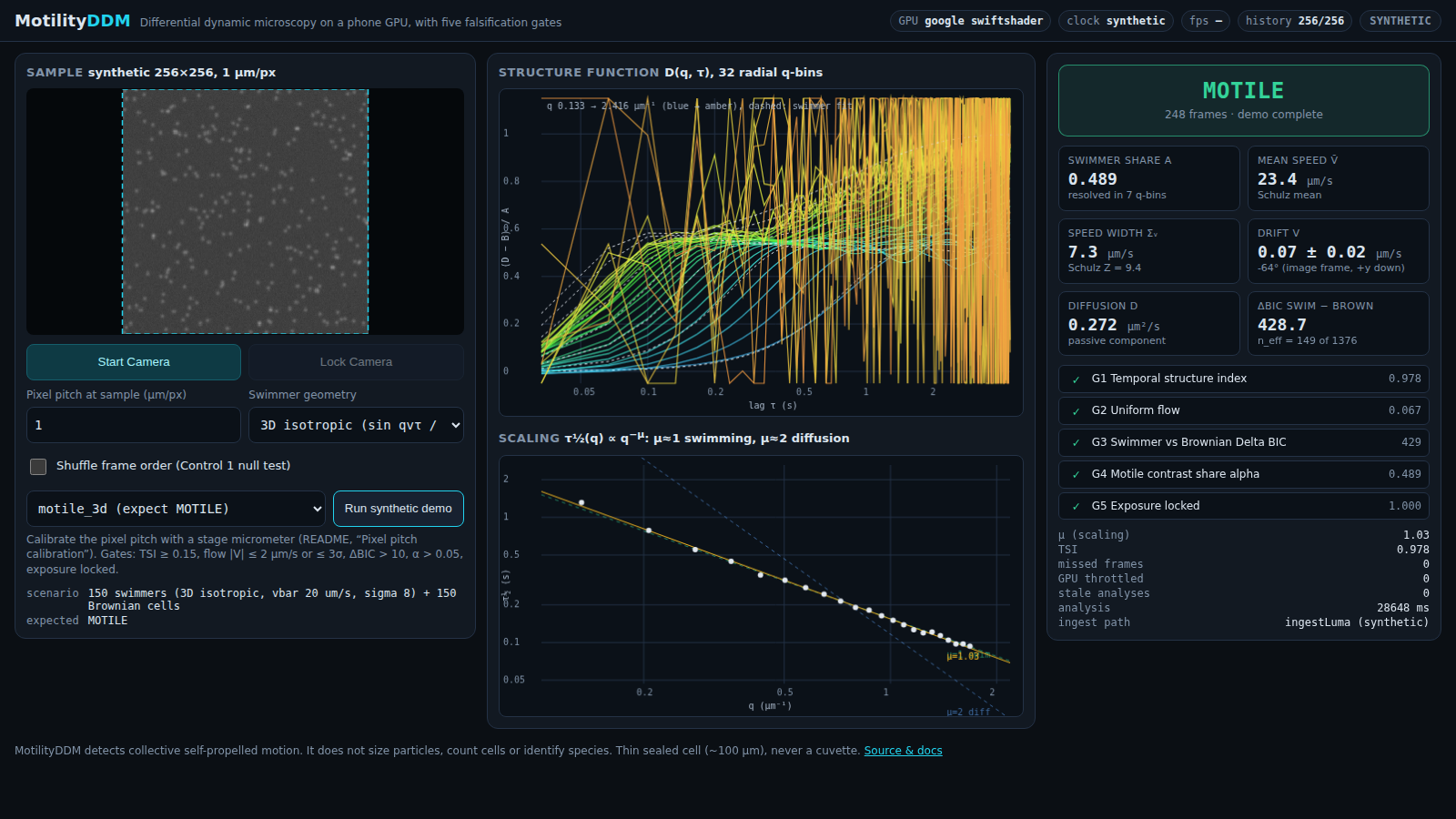
The part that really drove the project was making a detector that can say no. Convection, drift, auto-exposure flicker and dead cells jiggling under Brownian motion all look like "movement". A motility detector that can't reject them is worse than none. So MotilityDDM is built around falsification: every "MOTILE" verdict has to survive five gates and three controls.
What it does
Phone B's screen is a diffuse backlight under a sealed 100 µm thin cell. Phone A films it through a clip-on macro lens. The app:
- Locks exposure, ISO, focus and white balance, then reads the registers back to confirm the lock.
- Streams the central 256 × 256 pixels of every frame into WebGPU and computes the 2D Fourier transform of all 33,024 modes over a 256-frame history.
- Computes the DDM image structure function $$D(q,\tau) = \left\langle \left| F(q,t+\tau) - F(q,t) \right|^2 \right\rangle_t = A(q)\,\big[1 - f(q,\tau)\big] + B(q)$$
- Fits a swimmer-plus-Brownian model and returns one of
MOTILE,NOT_MOTILE,DIRECTED_TRANSPORT,NO_DYNAMICSorUNLOCKED_EXPOSURE.
Swimmers decorrelate ballistically, \( \tau_{1/2} \propto q^{-1} \), while diffusion gives \( \tau_{1/2} \propto q^{-2} \). The dashboard plots both live.
How we built it
GPU pipeline (WGSL, WebGPU). Six compute kernels:
ingest,reduce_mean,fft_rowsandfft_colsrun on every frame (radix-2 Stockham FFTs in workgroup memory).temporalis a masked Wiener–Khinchin estimator, split into 8 dispatches of 4,128 workgroups.radialreduces the results into 32 q-bins plus the phase-drift sums.
Everything fits inside default WebGPU limits: a 67.6 MB history buffer and 10 KB of workgroup memory. Dropped frames are masked, never interpolated, using exact pair counts \( N(\tau) \): $$D(\tau) = \frac{A(\tau) + A(-\tau) - 2\,\mathrm{Re}\,G(\tau)}{N(\tau)}, \qquad G = \mathcal{F}^{-1}!\left(|\mathcal{F}(m\,x)|^2\right)$$
Physics. We use Wilson et al.'s intermediate scattering functions with a Schulz speed distribution. Both have closed forms:
- 3D: \( \langle \sin(qv\tau)/(qv\tau) \rangle \)
- 2D: \( \langle J_0(qv\tau) \rangle \), via a Legendre function of real degree
The model is $$D_b(\tau) = A_b\left[1 - e^{-Dq^2\tau}\,J_0(q|V|\tau)\big((1-\alpha) + \alpha\, g(q\bar v\tau)\big)\right] + B_b$$ The amplitudes are solved exactly by NNLS inside every objective evaluation (variable projection), so the nonlinear search only sees \( (\bar v, Z, D, \alpha) \).
Falsification gates.
- A temporal structure index rejects static or shuffled movies.
- A uniform flow is measured directly from coherent Fourier phase rotation, \( \arg[C(\tau+1)\bar C(\tau)] = -\mathbf{q}\cdot\mathbf{V}\,\Delta t \).
- The swimming model must beat pure diffusion by \( \Delta\mathrm{BIC} > 10 \).
- The swimmer contrast share must satisfy \( \alpha > 0.05 \), with the swimmer decay actually resolved.
- Exposure must be verifiably locked.
Verification. Every GPU kernel has a float64 JavaScript twin with the same memory layout.
- A parity harness compares 4.2 million values element by element against the reference.
- An 11-scenario simulator covers motile, sparse, killed, static, shuffled, three flows, slow drift and 20 % dropped frames. It runs the full pipeline end to end, and all 11 are classified correctly.
Challenges we ran into
- BIC was lying to us. Our first model gave pure Brownian data a ΔBIC of +523 in favour of "swimming". Two things caused it. Residuals across lags are strongly correlated (\( \rho \approx 0.7 \)) because every lag reuses the same frames. And a per-bin swimmer amplitude gave the model 34 extra parameters to soak up noise. We switched to one physical, q-independent \( \alpha \) and an effective sample size \( n_\text{eff} = n(1-\rho)/(1+\rho) \). Null runs now sit near ΔBIC ≈ −15, and motile runs above +277.
- A slow 1 µm/s drift read as MOTILE. A radially averaged drift, \( J_0(qV\tau) \), is mathematically a 2D swimmer with a single speed. The fix was to measure V from Fourier phases, compensate it in both models, and add a 2 µm/s floor below which no "swimmer" can be claimed.
- f32 precision on the GPU. A single-pass f32 mean leaked into the low-q modes through the window sum, giving a spectral error of 2.6 × 10⁻⁴ against a 10⁻⁴ budget. Storing the mean as an f32 (hi, lo) pair brought it to 1.2 × 10⁻⁵. We also moved the mask spectrum and the twiddle factors to float64 on the host, so no kernel depends on the GPU's
sin/cos. - "A valid external Instance reference no longer exists." We reproduced this crash and reduced it to a 16 × 16 test case. The software GPU (SwiftShader) can't import any video frame into WebGPU. We kept the zero-copy camera path, added a canvas-readback fallback for broken drivers, and left the camera-import step to be validated on real hardware.
- Physics of the cell. A phone screen under the sample heats it from below, which is the classic Rayleigh–Bénard setup. A 1 cm cuvette reaches \( Ra \approx 1.5\times10^4 \) and convects. Because \( Ra \propto h^3 \), a sealed 100 µm cell is \( 10^6\times \) lower (\( Ra \approx 0.015 \)), so it doesn't.
What we learned
- Detecting something is easy. Defending the detection is the real work: controls, null models and honest statistics.
- Correlated residuals quietly break textbook model selection.
- WebGPU is ready for real scientific computing on phones, as long as you respect f32 precision and resource lifetimes.
Accomplishments and honest status
- CPU: 117 unit checks pass, and all 11 validation scenarios are classified correctly.
- GPU parity on a software GPU: spectrum error 1.2 × 10⁻⁵, D(q, τ) p99 9.9 × 10⁻⁷, and the same verdict as the reference.
- Not yet done: desktop and phone GPU runs, and live-sample measurements, are logged in
docs/DEVICE.mdas pending. The samples in our video are simulated and labelled as such. - Scope: MotilityDDM does not size particles, count cells or diagnose anything.
What's next
- Run the hardware protocol on target phones.
- Film the three live controls (frame shuffle, bleach kill switch, induced flow) on real samples.
- Deploy to GitHub Pages so anyone with two phones can try it.
Built With
- android
- canvas
- chromium
- css3
- differential-dynamic-microscopy
- esbuild
- fft
- html5
- javascript
- mediastream-api
- node.js
- playwright
- typescript
- vite
- web-workers
- webgpu
- webrtc
- wgsl


Log in or sign up for Devpost to join the conversation.