MNIST BNN

INSPIRATION

The idea came from a simple question: what is the smallest, most stripped-down version of a neural network that could still do something real? MNIST digit classification is the classic benchmark .. ten classes, 28x28 images, a problem solved daily in software in milliseconds. The challenge was whether we could implement it not in software, not in an FPGA fabric that hides complexity behind lookup tables, but as actual synthesised logic destined for a real silicon die through the Tiny Tapeout shuttle.

Binary Neural Networks were the answer. By constraining every weight and activation to a single bit (±1, represented as 0/1), multiplication collapses to XNOR and accumulation becomes popcount, operations that map directly to gates with almost no overhead. The prospect of running a trained neural network as pure combinational and sequential logic, with no CPU, no memory controller, and no floating point, was what made this worth doing.

HOW IT WAS BUILT

The network is a three-layer pipeline trained in Python with TensorFlow, then exported to hardware.

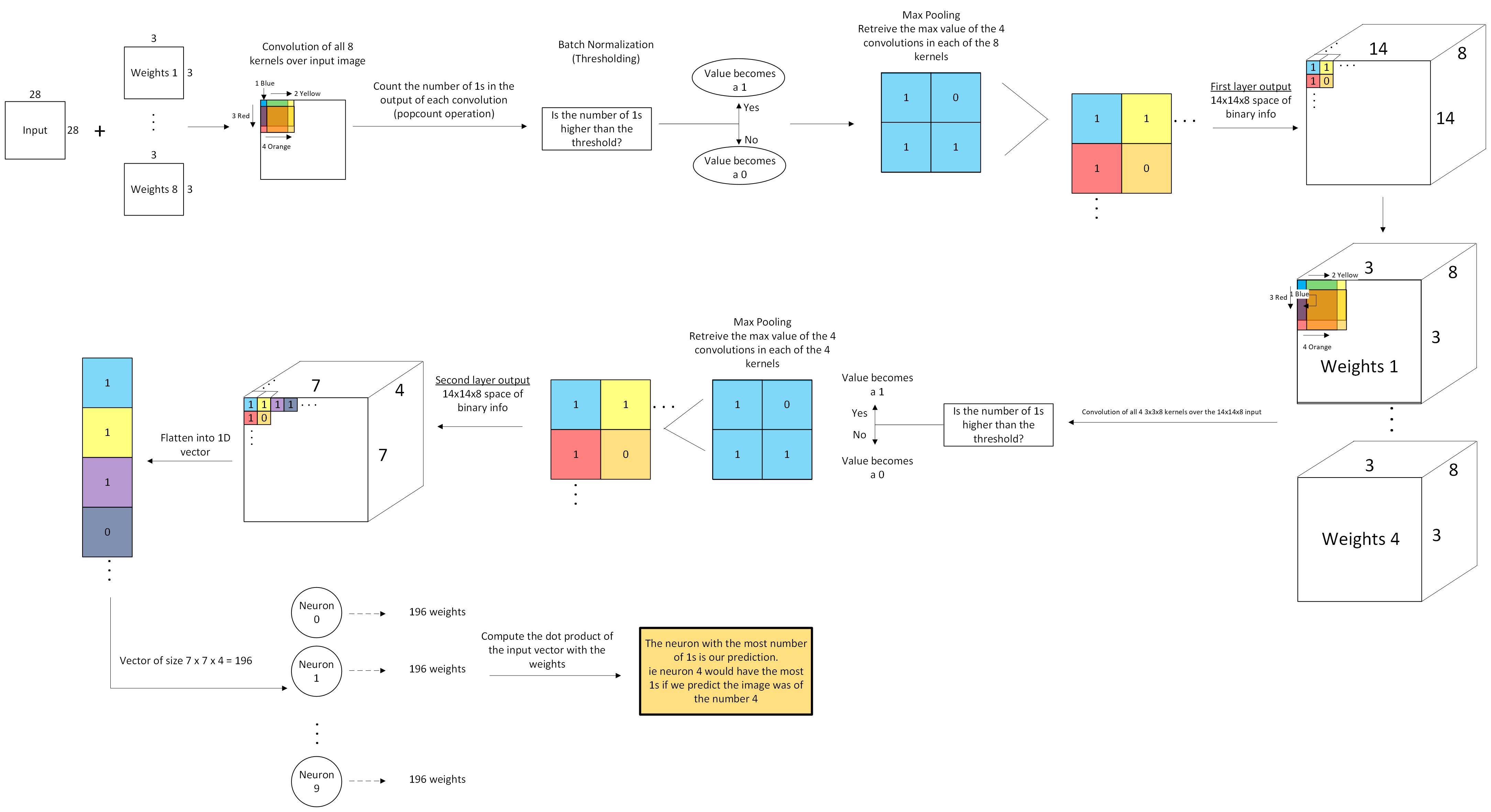
Training: Weights were trained with binarized activations. Batch normalisation layers in the Python model serve a dual purpose: during training they stabilise gradients; after training their learned scale and bias are folded into a single integer threshold per filter. At inference time, "does the popcount exceed the threshold?" replaces the entire batch-norm + activation computation.

Layer 1 — 8 filters, 3×3 kernel, 1 input channel → 72 weight bits Layer 2 — 4 filters, 3×3 kernel, 8 input channels → 288 weight bits Layer 3 — 10 neurons, 196 inputs each → 1960 weight bits

Total: 2320 weight bits loaded serially at startup.

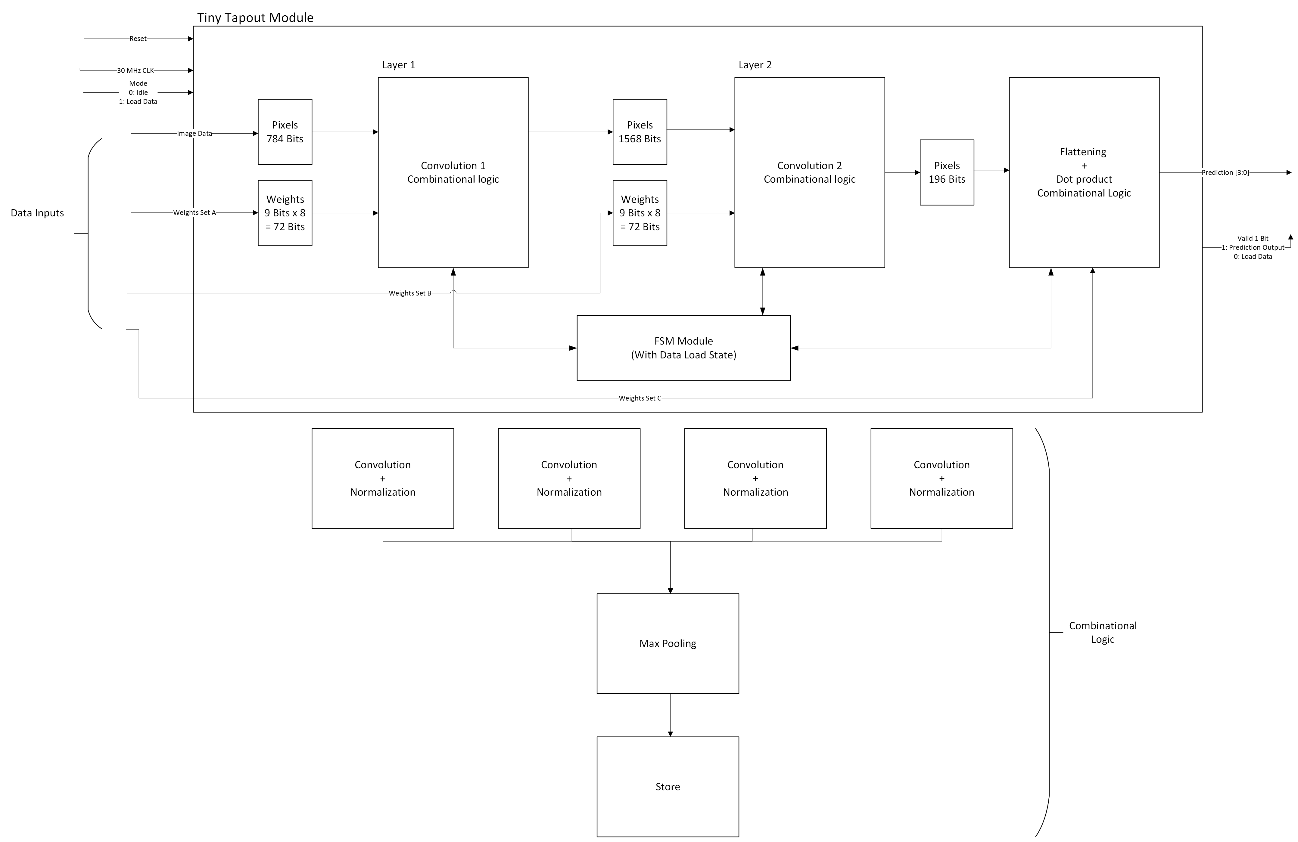
Architecture: The hardware is organised around a five-state FSM:

IDLE → LOAD → LAYER_1 → LAYER_2 → LAYER_3

LOAD: Pixel bits (784) and weight bits (2320) are clocked in simultaneously on two dedicated input pins. Three sequential always-blocks in registers.sv fill the weight registers for each layer in order, gated by completion flags (w_done, w_done1, w_done3), so the single serial weight pin feeds all three layers without multiplexing logic in the testbench.

LAYER_1: One output pixel is computed per clock cycle using combinational XNOR convolution over the 28×28 input. Eight filters produce a 14×14×8 feature map after 2×2 max-pooling. The popcount is compared to a hardcoded per-filter threshold derived from batch normalisation.

LAYER_2: The same pattern repeats over the 14×14×8 feature map, producing a 7×7×4 output — 196 bits total.

LAYER_3: A single-cycle combinational dot product (XNOR + popcount) across all 196 inputs for each of the 10 output neurons. A winner-takes-all comparison tree selects the neuron with the highest popcount, and its index appears on uo[3:0].

A reset synchroniser (reset_pipe.sv) converts the asynchronous rst_n into a clean synchronous reset that propagates through all modules, avoiding metastability at reset release.

Verification: Testing was done at multiple levels. Individual module testbenches (layer_one_tb, layer_two_tb, flatten_layer_tb, fsm_tb) were used during development. The top-level cocotb test in test/test.py drives the full design through the TinyTapeout interface and checks both that the output is a valid digit and that it matches the expected label from the verifying dataset.

A plain-Icarus testbench (top_test_tb/tb_top.sv) was added to run batches of real MNIST images without cocotb, loading pixel and weight data from .mem files generated by gen_real_mnist_images.py. This made it easier to sweep many images quickly and identify which specific dataset indices pass or fail.

WHAT WAS LEARNED

1. Bit ordering is everything in serial hardware. The single most time-consuming debugging task was tracing mismatches between the Python training code's weight layout and the order in which the hardware shift registers absorb bits. A one-bit offset anywhere in a 2320-bit stream corrupts every subsequent weight.

2. Combinational output registers behave differently from what you expect. layer_one_out and layer_two_out are declared as reg but written in always @(*) blocks — one bit at a time as the FSM scans through positions. This means they are not fully latched; unvisited bits retain their previous value. The design is still correct because every bit is overwritten before the done signal is asserted and the next stage reads the output, but it was a source of confusion when inspecting waveforms mid-computation.

3. Reset synchronisation matters even in simulation. The reset_pipe module ensures that synchronous_reset deasserts on a clock edge, preventing glitches on FSM state. An early version connected the flatten layer directly to raw rst_n rather than synchronous_reset, causing it to exit reset two clock cycles before the FSM — harmless in this design but indicative of the kind of subtle timing bug that becomes catastrophic in silicon.

4. Batch normalisation thresholds must be recomputed, not just exported. The Python thresholds are derived from the model's running statistics and must be re-evaluated after weight binarisation. Using pre-binarisation thresholds gave a model that looked correct in software but performed poorly in hardware.

5. Tiny Tapeout's eight-pin interface forces creative I/O design. With only ui[7:0] available, every pin carries multiple meanings across FSM states. Mode, pixel, and weight data share three pins, which is manageable — but any future expansion (e.g. streaming output probabilities rather than just the argmax) would require protocol changes.

CHALLENGES

Accuracy on the verifying dataset is lower than expected ... The most likely causes, in rough order of suspicion:

• Weight bit ordering mismatch between Python and the hardware shift registers. The training scripts and the registers.sv loading order were aligned iteratively, but a systematic off-by-one in any loop bound could explain a large accuracy drop without producing obviously wrong waveforms.

• Threshold values. The per-filter thresholds hardcoded in layer_one.sv and layer_two.sv were derived from one training run. If the weights were retrained or quantised differently in a later iteration, the thresholds would need to be updated to match.

• The verifying dataset itself may have a different distribution than the training set for the binary representation used here. Images that are borderline in the binarised domain are disproportionately likely to fail.

• Simulation vs. silicon: the cocotb test and the iverilog testbench both agree on results, which at least rules out a simulator-specific bug. The design has not yet been tested on actual hardware.

Despite the accuracy gap, the project achieved its core goal: a fully serial- loadable binary neural network, synthesisable to real silicon, that correctly classifies a meaningful fraction of handwritten digits with no CPU and no floating-point logic .. just gates.

Built With

• python
• systemverilog
• tensorflow
• verilog