hpcp | Devpost

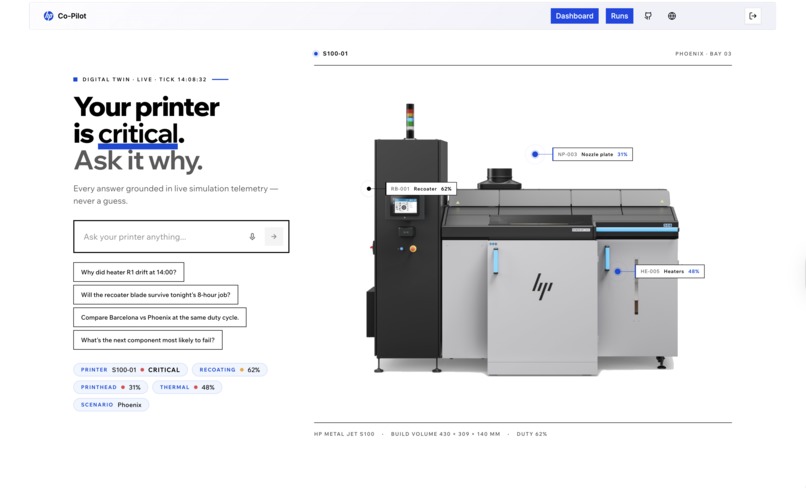
concept
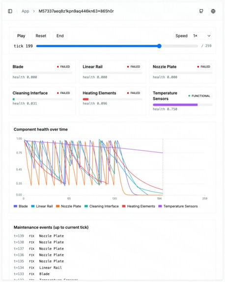
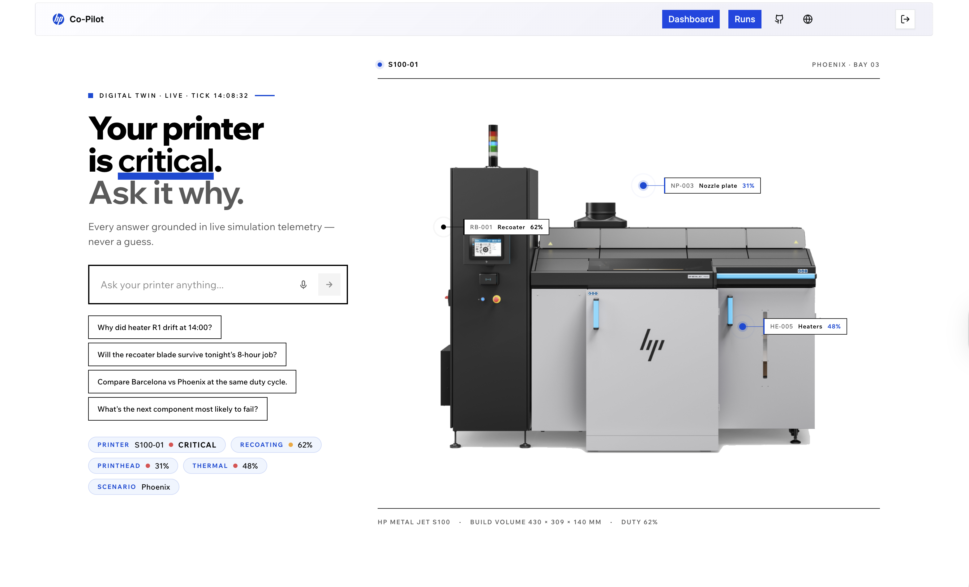
simulation dashboard
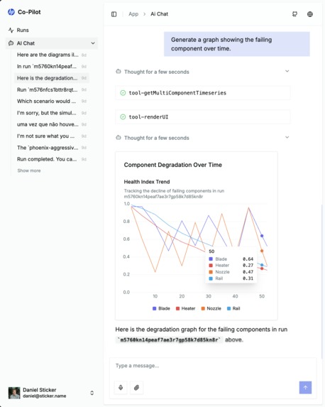
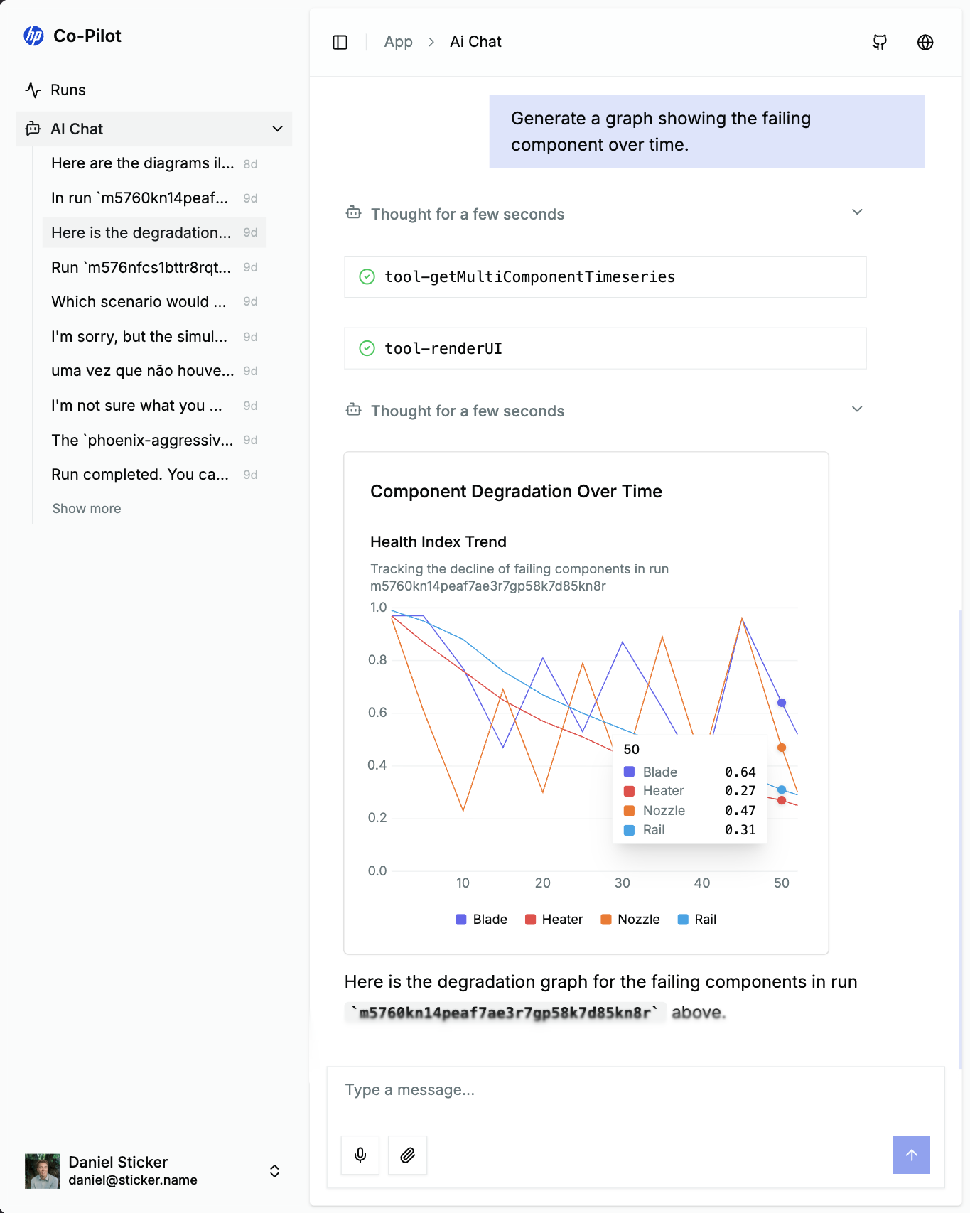
agent generating a custom graph
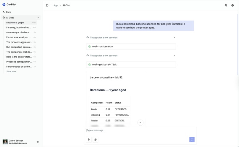
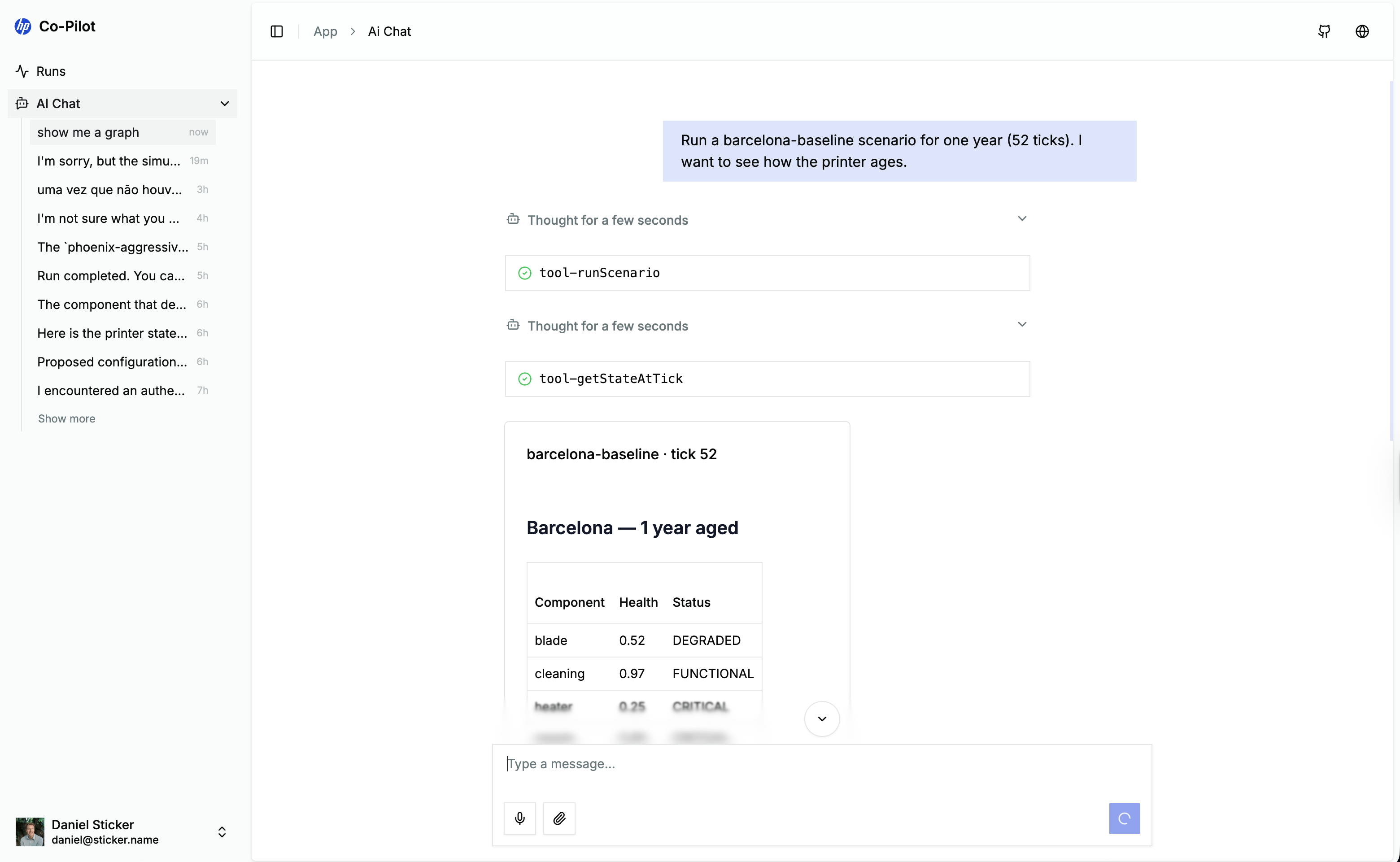
agent interface

Problem

HP's brief asked for a co-pilot for the Metal Jet S100, an industrial binder-jetting printer that sinters metal parts over hours of layered powder spreading. Components age, climates differ, sensors lie. The deliverable was a physics model, a simulator that advances time and persists state, and a grounded language interface that never invents a number.

Architecture

A coupled discrete-time system over six components across three subsystems. One tick is one simulated week.

Each tick, Engine.step(prev, drivers, env, dt) builds an immutable CouplingContext from the t-1 snapshot, then steps every component from the same frozen view (sim/src/copilot_sim/engine/engine.py). Update order cannot perturb the result. Per-tick stochasticity flows through derive_component_rng(scenario_seed, tick, component_id) keyed by a blake2b digest, so the historian is byte-identical across machines.

Two state objects come out: PrinterState (true) and ObservedPrinterState (sensor-side). The maintenance agent and chat layer only read the observed one.

Six components, four physics laws

Recoater blade

The recoater blade ages by Archard's classic abrasive law V = k F s / H, split across the four drivers (sim/src/copilot_sim/components/blade.py). Each tick:

$$ \Delta w = w_0 \cdot (1 + 0.10\,T_{\text{eff}}) \cdot (1 + 0.5\,H_{\text{eff}}) \cdot (1 + 0.6\,L_{\text{eff}}) \cdot \frac{h_{\text{week}}}{60} \cdot (1 - 0.8 M) \cdot \Delta t $$

where w_0 = 0.04 per week. Hot beds soften hardness H. Humid powder grits amplify k. Heavy queues raise contact force F. Phoenix runs 110 h/week against Barcelona's 60.

Linear rail

Rolling-element bearings fail as L_{10} \\propto (C/P)^3, so we keep the cubic Lundberg-Palmgren exponent visible in the load amplifier (components/rail.py):

$$ \Delta D = D_0 \cdot (1 + 4 L_{\text{eff}}^3) \cdot (1 + 0.10\,T) \cdot (1 + 0.40\,H) \cdot (1 + 0.5 v) \cdot (1 - 0.8 M) \cdot \Delta t $$

with D_0 = 0.012/week, vibration term v from the per-scenario Environment. A Weibull baseline R(t) = \\exp(-(t/\\eta)^\\beta) (η = 77 weeks, β = 2.0) multiplies into the final health.

Nozzle plate

Two damage processes run in parallel (components/nozzle.py). Thermal fatigue uses Coffin-Manson cycles-to-failure N_f = (\\varepsilon_0 / \\Delta\\varepsilon_p)^{1/c} with c = 0.5, accumulated under Palmgren-Miner:

$$ \Delta D_{\text{fatigue}} = 0.04 \cdot (1 + T_{\text{eff}} + b_{\text{heater}}) \cdot (1 + 0.5 L) \cdot (1 + 0.20 H) \cdot \frac{h_{\text{week}}}{60} \cdot (1 - 0.8 M) \cdot \Delta t $$

In parallel, a Poisson clog hazard fires each tick:

$$ \Delta n_{\text{clog}} \sim \text{Poisson}(\lambda \Delta t), \quad \lambda = 0.05 \cdot (1 + 4 H_{\text{eff}}) \cdot (2 - \eta_{\text{clean}}) \cdot (1 - 0.8 M) $$

A degraded cleaning interface roughly doubles the arrival rate.

Heater and PT100 sensor

Resistance drift on Ni-Cr elements (E_a = 0.7 eV, T_ref = 423 K) follows Arrhenius and accelerates with operating temperature (components/heater.py, components/sensor.py):

$$ AF = \exp\!\left( \frac{E_a}{k_B} \left( \frac{1}{T_{\text{ref}}} - \frac{1}{T_{\text{op}}} \right) \right) $$

$$ \Delta\rho = 0.0035 \cdot AF \cdot (1 + 0.3 T) \cdot (1 + 0.5 H) \cdot (1 + 0.4 L) \cdot (1 - 0.8 M) \cdot \Delta t $$

T_op = T_ambient + 130 \\cdot L_{eff} + 273.15 ties the ambient driver back through engine.coupling.ambient_temperature_C_effective. The PT100 uses the same AF to grow its bias_offset, with a hard FAILED gate at |bias| > 5 °C.

Cascading failures

Ten named factors live in CouplingContext.factors (engine/coupling.py). Every cross-component effect routes through them.

A blade wears. humidity_contamination_effective rises by 0.20 \\cdot blade\\_wear. Dirty powder feeds the nozzle's Poisson clog rate. Clogs raise operational_load_effective, which raises heater duty, which accelerates Arrhenius drift on heater and sensor alike. The drifting PT100 reads low, the controller over-shoots, each layer cure is hotter than commanded, and heater_thermal_stress_bonus enlarges the nozzle's Coffin-Manson plastic strain. The loop closes on itself.

True state vs observed state

The brief's most interesting clarification: not every component carries a sensor, and the ones that do can themselves degrade. build_observed_state in engine/assembly.py walks each component's SensorModel and produces observed_health_index, observed_status, and a sensor_note of ok | noisy | drift | stuck | absent. When too many sensors are missing or stuck, observed_status becomes UNKNOWN.

The maintenance agent only reads observed. A drifted PT100 can fool it exactly the way it would fool a human operator.

Maintenance agent

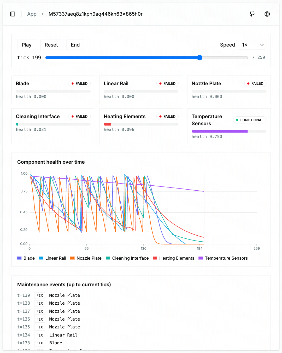
HeuristicPolicy.decide(observed, tick) (policy/heuristic.py) runs three rules in order: any UNKNOWN triggers TROUBLESHOOT; otherwise the lowest observed health below 0.45 gets FIX (or REPLACE below 0.20), worst-first; otherwise a monthly preventive FIX of the longest-untouched component. Maintenance is applied between ticks, never inside a step. Same seed, three policies (no-agent, heuristic, LLM-as-policy) produces a clean A/B chart of min(component_health) over 180 days.

HP Copilot chat layer

A Convex agent (@convex-dev/agent, OpenRouter, Gemma 4-31B) with nine tools over the SQLite historian: listMyRuns, getRunSummary, getStateAtTick, getComponentTimeseries, getMultiComponentTimeseries, listEvents, inspectSensorTrust, compareRuns, runScenario (web/src/lib/convex/aiChat/agent.ts, web/src/lib/convex/sim/tools.ts). Every printer-state claim must cite runId, tick, and componentId from a tool result. The agent renders structured cards via a renderUI tool with a strict shadcn schema. inspectSensorTrust is the diagnostic that separates a component fault from a misled sensor.

Stack

Python 3.12, NumPy, FastAPI, Docker, SQLite (WAL) for the sim and historian. Streamlit for the initial dashboard draft and simulation iteration. SvelteKit + Convex + OpenRouter (Gemma) for the operator chat. Synthetic temperature and humidity drivers calibrated to Barcelona vs Phoenix climate.

What's next

Auto-tune the per-component physics parameters from real sensor streams. The law shapes are right (Archard, Coffin-Manson, Arrhenius); their coefficients are hand-calibrated. Hooking the historian schema up to a fleet of running Metal Jet S100s would let the agent fit k, D_0, E_a, and the cascade gains per machine, then ship realistic per-unit predictions instead of scenario-shaped ones.