Inspiration
In times where there is an ample amount of spectroscopic data available and the GAIA satellite (measuring stellar fluxes, measuring the distances, and most importantly for us: Taking spectra for some of them). Given the incredible data volume this satellite mission provides the community, there is simply not enough manpower to analyze all these spectra by hand. Of course, other (spaceborne) observatories may create datasets which extend to a size a single human cannot grasp. Since Fraunhofer systematically characterized the solar spectrum and we advanced to the state-of-the-art technology we have available today, it is of the oldest ideas and disciplines to find patterns in how stars and celestial objects behave or look like. Many decades ago, scientists started to categorize stars according to their spectral appearance. We later learned that the spectral classification like still we use today, a.k.a. The OBAFGKM-sequence indeed tells us about some physical properties of the respective stars like their metal content, surface pressure, and temperature! In the times of big data, we try to reach for higher and higher degrees of automation. In the spirit of combining astrophysics with machine learning, in the scope of this project, we developed the fundamentals towards a machine learning-driven. Our result that we like to share with you is just a first step towards a fully-automated determination of spectral classes that can allow the big data-addicted astrophysicist to spend more time to brew as fresh mug of coffee to stay awake during and observe night rather having to deal more monotonous manual, classification of their subject. ;D :wink:
What it does
We use a decision tree based Machine Learning algorithm. We classify the spectral type of the star with respect to their absorption spectral lines.
The guiding problem is basically analogous to ask about the age of a human: Describing to an alien that doesn’t know how human evolution works could pose some challenges in principle. They are actually of the same nature like the one, we are dealing with here. To estimate a human’s age, one could evaluate features in their appearance like (amount of wrinkles, body size, …). We then also need to specify certain age categories, each of which have a unique combination of characteristics. The same idea we apply to the stars that we are looking at. A priori, we (or the machine) do not not know what a stellar spectrum tells about the stellar surface temperature. However, we can define a set of characteristics (in this context spectral absorption features) which hint towards certain stellar temperature regimes based on their presence and absence. Like a rather old human would have lots of wrinkles and gray hair, cooler stars may exhibit molecular absorption bands like titanium oxide in their spectra, whereas hotter stars rather show strong absorption in ionized helium.
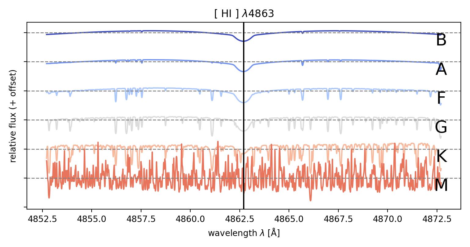
The absorption lines indicate the presence of certain elements/molecules in the immediate vicinity of the star. They are formed when photons of a particular wavelength from the stellar interior are absorbed by the electrons of the elements/molecules which then in return are being excited to a higher energy state. These lines happen to appear at distinct wavelengths as their formation is only possible by unique electron transitions in specific elements/molecules, therefore these provide us the abundance of an element/a molecule in the given star. The relative strength of different absorption lines are excellent indicators for the temperature of the visible regions of the star. The more hotter the star, the absorption lines from primordial elements like Hydrogen and Helium are observed more in the spectra compared to relatively cooler stars which has the presence of absorption line caused by molecules and metals (in astrophysics, any element beyond Hydrogen and Helium come under the broad category of metals).
The Standard classification system that is widespread in the field of astrophysics is the Morgan - Keenan (MK) classification. This was developed by the infamous “Harvard Computers” in the early 20th century. The categories are as follows: O,B,A,F,G,K,M, where the temperature of the stars drops from left to right across the classes (check out this page to learn more on the fundamentals of classification: link). The classification is dependent on the strength of the absorption lines. Strength of the absorption is a direct indicator of the abundance of the element/molecule which is responsible for it and this information enables us to find the temperature of the system and therefore the spectral class.
Through MLoL we explore the possibility of using Machine Learning to determine the spectral type of the star without human bias. The strength of an absorption line could be inferred to have different strengths across individuals (especially those who are relatively new to absorption lines spectrography) and might lead to misclassification of the star’s spectral type. Also with the abundance of data that is at our disposal, it is wise to automate the classification of the stellar spectra. With Machine Learning Algorithm, the strength of the absorption lines are treated numerically and the classification proceeds from an algorithm that the Machine Learning routine self learns from the given parameters. When we proceed to do the classification using the strength of the absorption spectral lines, we tend to categorize the depth of the absorption line (lowest flux value) as the strength but the depth of the absorption lines are sensitive to the noise and varies significantly with noise. Therefore the width of the absorption line would be the best way to classify the spectral type. But to use the width as a marker of strength for the absorption line, it is normalized before the data analysis.
The spectrum is normalized by creating a continuum from the given spectra and using it as the baseline to normalize the flux of the spectrum. The width of the absorption line can be expressed by the area of the region bounded by the inverted cone of the absorption line and the normalized flux line. This value is reliable despite the presence of noise, if any. The Machine Learning routine, which is a tree based algorithm, is trained by the PHOENIX dataset for the spectral class B to M, and learns to classify the spectral type of the stars through the given parameters (area of the absorption line in normalized spectra) through a “blackbox” algorithm, developed from the linkage it learns from the training dataset.
Once this is done, we test it with spectra of the known stars like Vega, Betelgeuse from UVES (VLT Telescope) and test the performance of the routine, after converting their spectra to normalized form by a self written, automated python script.
How we built it
The Program runs on Python and uses a variety of libraries/packages available. At its heart, the machine learning algorithm decides on the spectral class upon the spectral features commonly known to be indicative for their respective spectral classes. To a certain degree, this program works like a data pipeline with the input of model spectra and the final output being the spectral class. However, there are numerous steps in between that we need to consider: Coming back to the fundamental problem: We start with a spectrum that we would like to analyze, so a spectrum, i.e. a tuple of arrays containing both wavelength and flux information mark the beginning of the entire process. The machine now expects two additional inputs:
- A list of lines that are indicative and unique to some extent for discriminating the stellar spectra into distinct spectral classes
- The spectra to which the test spectra will be compared to in the end Both of them provided, the routine will start to figure out what the spectral class-characteristic absorption features look like. Based on this, it will determine the absorption strength at each of these lines. With this, the algorithm creates a model to which the test spectra will be compared to. When providing the test spectrum the machine will decide in which spectral class the test star fits the most. As the program already did for the training spectra, it initiates the data reduction process by evaluating the absorption lines strengths at the same wavelengths as specified in the file containing the list of characteristic absorption transitions. Given the absorption strengths of the test spectrum, it can then directly compare the line strengths to the parameter space given for the model’s training. What is the result of this: A spectral classification 100% based on comparing spectra with machine learning algorithms. Voila!
The Machine Learning routine was built using the “tree” module of the “sklearn” package using python. Sklearn is a widely used package exclusively for machine learning related applications. The DecisionTreeClassifier function is the primary function which is used to train the algorithm. The training is done with Decision Tree Algorithm as Decision Trees are well acknowledged for classification problems under given conditions. The way that the routine learns to classify is a blackbox which prevents any preference bias or weightage to the parameters that we have, and therefore you have a generalized analysis of the spectral class from the absorption line strength. We have limited our analysis only in the visible region of the electromagnetic spectrum.
Challenges we ran into
A very fundamental challenge we were exposed to was the search for an appropriate database that could provide us an easy-access for spectra to analyze. Due to this project being limited to 24 hours only, we had to make sure that the spectra have a consistent data format in order to save time and not spend too much time looking at each spectrum individually. We base our training on models generated with stellar structure codes. Alongside, we also consider real observational data for the refined calibration and cross-check of the results which we obtain using our method using instrumental output from the UVES Spectrograph (@VLT). Initially, we tried to build our training set in a way such that it is based on the cross-correlation data templates from the Sloan Digitized Sky Survey (SDSS). Though, we were having issues with finding a correct wavelength scale as the data in the FITS header did not produce meaningful spectral axes. For instance, as we tried to build the spectra from the data, we found H-alpha absorption to be located around ~6200 Angstrom. This is far away from the rest wavelength of this transition at about 6562 Angstrom. After a loss of some time we eventually considered basing our training model on the PHOENIX spectra. This has the major advantages of
- … them providing very high-resolution spectra without instrument-based noise (like thermal noise a CCD detector would introduce → this makes it easier to identify and measure the spectral lines
- … them covering an exceptionally wide spectral range which covers all of our spectral lines features whose intensity we use as tracers for the spectral type
Especially cooler stars intrinsically have a plenty of absorption features such that it is hard to avoid misinterpretation of lines that are physically independent of the one we are looking at, but happen to appear close to the actual lines of interest on the wavelength axis. In a more technical context, it turned out to be challenging to perform the baseline fitting of the lines. While for the most narrow and weak absorption features, the baseline fit performed pretty well, especially the deep, wide, and winged hydrogen absorption features gave us a hard time. For the algorithm, it was hard to see where the absorption profile ended and where the actual continuum begins. For those lines, their absorption depths in absolute terms is, therefore, hard to be determined to an acceptable extent.
Accomplishments that we're proud of
Some of the key features:
- Normalization of stellar spectra on narrow wavelength bands in the immediate vicinity of spectral features (i.e. useful to perform baseline normalization)
- High-level comparison of model spectra to observations.
- In less than 24hrs: Get to know a lot of different file formats from various instruments and understand the data architecture of them
- We have meticulously worked on developing the training dataset with wavelength and area occupied by the absorption lines which is one of its kind as it is not available in any other database across the internet.
- We developed our approach in such a way that we didn’t have to work on hundreds of spectra to train the ML routine but used a powerful catalog which yields us the same results.
- The first results we got were quite promising! For instance, we tested UVES spectra for Betelgeuse and Vega both of which have well-known spectral classes. To mention one of the preliminary results: Vega has an inherent spectral class of A0 (and is also the reference source in a lot of disciplines) and the ML approach yielded spectral classes of A and G in two runs. In addition testing Betelgeuse which is a red supergiant with the spectral class M2, our approach predicted it to be of spectral class K or M. In both examples, the predicted spectroscopic types are close or even matching to the literature values. This is impressive, given that we achieved to read out the fluxes, and involve stellar models within the given time of 24h. Even though our approach involves a lot of caveats to this point, it motivates us to take this project further and see in which aspects the machine’s decisions can be refined, yielding ever more precise results.
What we learned
- Different data structure and the benefits with each of them in niched operations
- Learnt ways to automatically downloading FITS file from online database and converting them into numpy.ascii file, ready to be used for data analysis
- The fundamental physics behind the spectral lines in the spectra and how depth and width of the spectral lines could be used to determine the strength of the absorptions lines
- How to make our raw data compatible with our Machine Learning Algorithm to train it but also to ensure that the train data and the test data are governed by the same parameters.
What's next for M-LoL (Machine Learning on absorption Lines)
- The PHOENIX database we found link gives a buffet of spectra with an enormous range of physical parameters like Metallicity, surface gravity, and most important for our 24h project: temperature. Due to the limited time frame we, had to restrict ourselves to the temperature (i.e. stellar spectral class) as the
- Improve the routine which determines the absorption strength. We just look for the minimum of the absorption in the close vicinity of the expected line center. This involves both ambiguities with noisy signals when moving the real observations, as well as breaks down as a good measure when entering the saturated line regime. The minimum fluxes at some point do not vary significantly anymore, once their minimum approaches 0. Fluxes less than 0 are unphysical!
- Increase the quantity of our test data
- Include more physics! So far, we only discriminate the stars according to their chromophoric temperature. However, there are more parameters, governing the spectral appearance of the star.
Built With
- python
- sklearn


Log in or sign up for Devpost to join the conversation.