\documentclass[11pt]{article}
\usepackage[a4paper,margin=1in]{geometry} \usepackage{amsmath,amssymb,mathtools} \usepackage{booktabs} \usepackage{enumitem} \usepackage{graphicx} \usepackage{hyperref} \usepackage{float} \usepackage{caption} \usepackage{setspace} \usepackage{microtype} \usepackage{xcolor} \usepackage{array}
\setstretch{1.08} \setlength{\parskip}{0.45em} \setlength{\parindent}{0pt}
\hypersetup{ colorlinks=true, linkcolor=blue, urlcolor=blue, citecolor=blue }
\title{\textbf{Cricket Match Simulation, Real-Time Win Probability, and Tactical Decision Support}} \author{LSE Traders} \date{}
\begin{document}
\maketitle
\begin{abstract} We build a ball-by-ball T20 cricket simulator that estimates live win probability from any intermediate match state. The simulator conditions on wickets in hand, overs remaining, player quality, venue effects, bowling resources, and tactical choices, then uses Monte Carlo continuation to produce full outcome distributions rather than point forecasts. It also supports counterfactual analysis: given the same match state, how does win probability change under different bowling or batting decisions? We calibrate the model on historical delivery-level data and evaluate it against both observed score distributions and held-out match outcomes \cite{akhtar2012,swartz2009,davis2014,perera2016,sharp2011}. \end{abstract}
\section{Introduction}
Static cricket forecasting models, like those based on current score or required run rate alone, miss an obvious problem: the same scoreline can mean very different things depending on who is batting, how many wickets are left, and who is still available to bowl. A team at 120/2 after 15 overs is in a much stronger position than one at 120/7, but a run-rate-only model treats them identically.
We address this by modelling T20 cricket as a state-dependent stochastic process. At each delivery, outcome probabilities depend on the full match state, including player identities, innings phase, venue, and bowling resources remaining. From any mid-match position, we simulate the rest of the match thousands of times to estimate win probability and score distributions \cite{akhtar2012,mchale2013,swartz2009,davis2014}.
The simulator has three components. First, a ball-outcome model that generates delivery results conditional on the current state. Second, a Monte Carlo engine that repeatedly simulates the match remainder to estimate win probability. Third, a tactical layer that compares alternative decisions (e.g.\ different bowling choices) from the same state and picks the option with the highest continuation win probability \cite{swartz2009,davis2014,perera2016,sharp2011}.
\section{Problem definition}
At any time (t), let the current match state be [ S_t = (\text{runs}, \text{wickets}, \text{balls remaining}, \text{target}, \text{striker}, \text{non-striker}, \text{bowler}, \text{conditions}, \text{resources left}). ]
We want to estimate [ P(\text{batting team wins} \mid S_t), ] and update it after every ball.
The difficulty is path dependence. As the example above illustrates, identical scorelines can imply very different winning chances depending on wickets in hand, who is at the crease, what bowling remains, and whether the venue favours batters or bowlers. A continuation-based probabilistic model handles this; a lookup table does not \cite{akhtar2012,mchale2013,swartz2009,davis2014}.
\section{Modelling framework}
We treat cricket as a discrete-time stochastic process observed ball by ball, following Swartz et al.\ \cite{swartz2009} and Davis et al.\ \cite{davis2014}, who model batting outcomes as conditional multinomial events indexed by player, wickets, overs, and score.
\subsection{State representation}
At ball (t), the game state is [ S_t = (\text{score}, \text{wickets}, \text{balls remaining}, \text{target}, \text{striker}, \text{non-striker}, \text{bowler}, \text{phase}, \text{venue}, \text{resources left}). ]
This state updates after every legal delivery.
\subsection{Ball outcome space}
Let [ Y_t \in {0,1,2,3,4,6,W,E (+\text{runs})} ] denote the outcome of ball (t), where (W) is a wicket and (E) denotes extras.
\subsection{State-dependent ball model}
Delivery outcomes are not drawn from a fixed distribution. Instead, [ P(Y_t = y \mid S_t, i, j, Z_t) ] depends on the current match state (S_t), the striker (i), the bowler (j), and contextual covariates (Z_t). This means the simulator behaves differently when a set opener faces a death-overs specialist than when a tailender faces the same bowler in the powerplay. Related state-dependent models appear in \cite{akhtar2012,swartz2009,davis2014,mchale2013}.
\subsection{Two-stage event decomposition}
We decompose the ball-outcome model into two stages for better interpretability and calibration.
\subsubsection*{Stage 1: Wicket model}
We first estimate the probability of a dismissal: [ P(W_t = 1 \mid S_t, i, j, Z_t) = \mathrm{logit}^{-1}(X_t^\top \beta). ]
Here, (X_t) includes innings phase, wickets in hand, required run rate, striker settledness, bowler spell length, venue baseline, and player-specific effects. Logistic models of this kind are standard in cricket forecasting \cite{akhtar2012}.
\subsubsection*{Stage 2: Run model conditional on survival}
Conditional on no wicket, we estimate [ P(R_t = r \mid W_t = 0, S_t, i, j, Z_t), \qquad r \in {0,1,2,3,4,6,E}. ]
Separating dismissal risk from scoring intensity lets us calibrate each component independently and diagnose where the model breaks down. Davis et al.\ \cite{davis2014} and Swartz et al.\ \cite{swartz2009} use similar conditional decompositions.
\section{Player effects and regularisation}
Rather than representing each player with a single rating, we use structured latent trait vectors. This is partly practical (a single number cannot capture the difference between a power hitter who is vulnerable to spin and a rotator who rarely gets out) and partly statistical (trait vectors allow the model to respond differently to different match situations).
\subsection{Batter traits}
Each batter is characterised by: strike rotation ability, boundary frequency, six-hitting power, dismissal resistance, pace effectiveness, spin effectiveness, death-overs acceleration, pressure sensitivity, settled-batter uplift, and a recent-form adjustment.
\subsection{Bowler traits}
Each bowler is characterised by: wicket-taking threat, economy control, boundary suppression, death-overs effectiveness, new-ball effectiveness, spin/seam profile, matchup strength, and fatigue resistance.
\subsection{Regularisation}
Raw historical rates are noisy for players with small samples. We shrink player-level estimates toward competition-level baselines: [ \hat{\theta}_i = \lambda_i \theta_i^{\text{hist}} + (1-\lambda_i)\theta^{\text{league}}, ] where (\lambda_i \in [0,1]) increases with sample size. A player with three T20 innings gets pulled heavily toward the league average; a player with 200 innings keeps most of their observed rates. This is the same logic as empirical Bayes shrinkage in hierarchical models \cite{davis2014,swartz2009}.
\section{Context and tactical state}
\subsection{Venue layer}
Each venue has a scoring baseline: [ V_g \sim \mathcal{N}(\mu_g,\sigma_g^2), ] where (g) indexes grounds. This lets the simulator distinguish, say, Chinnaswamy (flat, high-scoring) from Chepauk (slow, lower-scoring). Venue effects have been shown to matter materially in both state-based outcome models and resource-based scoring adjustments \cite{akhtar2012,mchale2013}.
\subsection{Latent pressure index}
We construct a pressure index from match-state variables: [ \text{Pressure}_t = f(\text{RRR gap}, \text{wickets left}, \text{balls left}, \text{bowling resources}, \text{venue difficulty}). ]
This enters the ball-outcome model as a covariate. The idea is simple: needing 12 an over with 8 wickets in hand is a different kind of pressure from needing 12 an over with 2 wickets in hand, even though the required rate is the same. Similar nonlinear interactions between wickets, overs, target, and run rate appear in \cite{akhtar2012,mchale2013,davis2014}.
\subsection{Settling-in effect}
New batters are temporarily less efficient and more dismissal-prone. As balls faced increase, performance approaches baseline ability: [ \Delta_{\text{settled},t} = \alpha \left(1 - e^{-k b_t}\right), ] where (b_t) is the number of balls faced by the striker.
\subsection{Bowler spell deterioration}
Bowler effectiveness can decline across long spells. We incorporate spell-length adjustments in both the wicket and run models, consistent with empirical work on bowling workload and physical load \cite{portus2000,constable2021}. In practice, this effect is small in T20 (bowlers bowl at most 4 overs). It would matter much more in ODI or Test cricket, where workload management is a genuine tactical concern.
\section{Strategy engine}
\subsection{Batting strategy states}
We allow batting intent to shift between four states: consolidate, balanced, accelerate, and all-out attack. These are inferred from match situation and recent scoring behaviour rather than set exogenously.
\subsection{Bowling strategy states}
Bowling tactics can reflect: wicket-seeking attack, run containment, saving death-over specialists for later, and matchup exploitation (where data permits). The choice between these is determined by the Monte Carlo engine: whichever bowling option yields the highest continuation win probability is preferred.
\subsection{Aggression index}
We quantify batting aggression using recent scoring relative to expectation: [ A_t = 0.5 z(\Delta \text{BoundaryRate}) - 0.3 z(\Delta \text{DotRate}) + 0.2 z(\Delta \text{WicketRisk}), ] where each term is measured relative to the expected rate conditional on state. This turns loose notions of ``intent'' into something the model can condition on. Empirically, T20 batting aggressiveness varies a lot by over, wickets lost, and target pressure \cite{davis2014}.
\subsection{Bowler selection as a decision problem}
At the end of each over, let (\mathcal{B}(S_t)) denote the set of bowlers still available under T20 constraints (each bowler may bowl at most 4 overs). The preferred choice is [ b^*(S_t) = \arg\max_{b \in \mathcal{B}(S_t)} \mathbb{E}\left[\text{WinProb after continuation} \mid b, S_t\right]. ]
This turns the simulator into something prescriptive rather than purely descriptive. Related optimisation formulations for cricket team selection use integer programming and simulated annealing over combinatorial action spaces \cite{sharp2011,perera2016}.
\section{Monte Carlo win probability engine}
Given a live match state (S_t), the estimation procedure is: \begin{enumerate}[label=\arabic*.] \item Freeze the current state. \item Clone it (N) times. \item Simulate each clone to completion, ball by ball. \item Record which side wins in each simulation. \end{enumerate}
If the batting side wins in (W) out of (N) simulations, the estimated win probability is [ \hat{P}(\text{win} \mid S_t) = \frac{W}{N}, ] with Monte Carlo standard error [
SE!\left(\hat{P}(\text{win} \mid S_t)\right)
\sqrt{\frac{\hat{P}(1-\hat{P})}{N}}. ]
Besides the point estimate, we also get the full score distribution, wicket distribution, percentile bands, best and worst plausible paths, and tactical counterfactual comparisons (by running the same procedure under different decisions). This continuation-based approach is the standard engine in cricket simulators \cite{swartz2009,davis2014}.
\section{Implementation}
The system is split into a Python simulation backend and a React frontend, connected by a FastAPI server. This section walks through each module and what it does.
\subsection{Data models (\texttt{models.py})}
All game entities are represented as Python dataclasses with continuous parameters. There are no discrete buckets anywhere in the model --- pitch pace is a float between 0 and 1, not a categorical label.
The \texttt{Player} dataclass carries batting ability, bowling ability, bowling style (pace, spin, or medium), aggression, consistency, fitness, and matchup preferences against pace and spin. Two derived properties matter most. \texttt{effective_batting} blends raw ability with recent form via an EMA multiplier: $\texttt{bat} \times (0.7 + 0.3 \times \texttt{form})$. The settling factor models the well-documented vulnerability of newly arrived batters: $1 - 0.35 e^{-b/8}$, where $b$ is balls faced. A batter who has faced 0 balls operates at 65\% of their steady-state ability; by 20 balls they are at 98\%.
\texttt{PitchProfile} and \texttt{WeatherProfile} encode venue and conditions as continuous floats. The pitch exposes derived modifiers: \texttt{pace_modifier} ($0.7 + 0.6p + 0.15b$, where $p$ is pace and $b$ is bounce), \texttt{spin_modifier} ($0.6 + 0.8s$), and \texttt{boundary_modifier} ($1.15 - 0.3g$, where $g$ is ground size). Weather contributes a swing boost from cloud cover and humidity, and a dew factor that accumulates over evening matches. The dew model is straightforward: zero before over 10 in day/night games, then $\min(1,\; 0.05 \times (\text{over} - 10))$. It dampens spin effectiveness and increases bowling pressure as the innings wears on.
\texttt{BallCondition} models the aging of the ball through the innings. Swing decays exponentially ($e^{-0.08 \times \text{over}}$), as does seam movement ($e^{-0.05 \times \text{over}}$). These feed into the bowler modifier functions in the sampler.
The \texttt{InningsState} dataclass tracks everything needed to simulate from any mid-innings position: score, wickets, legal balls bowled, batter innings records, bowler spell records, fall-of-wicket log, current pressure state, and batting intent. Its \texttt{clone()} method (a deep copy) is what makes Monte Carlo continuation possible --- we freeze the state, copy it $N$ times, and simulate each copy independently.
Ten international T20 squads are hard-coded with hand-calibrated player ratings (India, Australia, England, Pakistan, South Africa, New Zealand, West Indies, Sri Lanka, Bangladesh, Afghanistan). Each squad has 11 players with realistic role distributions: openers, middle-order batters, all-rounders, wicketkeepers, and specialist bowlers. The ratings reflect approximate current international standing and were cross-checked against career T20I statistics.
\subsection{Ball-by-ball sampler (\texttt{sampler.py})}
This is the core probability engine. Every delivery, the sampler computes a 9-dimensional probability vector over the outcome space ${0, 1, 2, 3, 4, 6, W, \text{Wide}, \text{NB}}$ and draws a single sample.
The computation has two stages. First, a set of base probabilities is generated by smooth interpolation across the innings. Rather than defining three discrete phase tables (powerplay, middle, death), the code parameterises outcomes as continuous functions of $t = \text{balls}/120$. For instance, the six-hitting probability follows $0.03 + 0.07 t^{1.5}$, which is low in the powerplay and ramps up through the death overs. Wicket probability follows $0.04 + 0.02t$, producing a modest increase as batters take more risks late in the innings.
Second, six modifier functions are applied multiplicatively:
\textit{Batter modifier.} Adjusts all outcomes based on the striker's effective batting ability (post-settling, post-form) and the pitch's batting and boundary modifiers. A batter with high aggression gets an amplified six-hitting multiplier; a batter with high consistency gets a reduced wicket multiplier.
\textit{Bowler modifier.} Adjusts outcomes based on effective bowling ability, bowling style, and conditions. A pace bowler on a pace-friendly pitch with cloud cover and a new ball gets compounded boosts to dot-ball and wicket probabilities. A spinner on a dew-affected evening surface gets the opposite.
\textit{Matchup modifier.} If the bowler is pace, the batter's \texttt{pace_preference} determines whether the matchup favours attack or defence. A batter with a pace preference of 0.8 against a pace bowler gets boosted boundary probabilities and reduced wicket probability; a batter with 0.2 (vulnerable to pace) gets the reverse.
\textit{Dual pressure modifier.} Both batting and bowling pressure affect the outcome vector simultaneously. High batting pressure (chasing team behind the rate, losing wickets) increases boundary attempts and wicket risk. High bowling pressure (batters ahead of the rate, few wickets taken) increases extras. The interaction captures what commentators call ``pressure from both ends'' in tight matches.
\textit{Fatigue modifier.} Bowler effectiveness degrades with balls bowled in the match, scaled by the bowler's fitness attribute. The effect is small in T20 (at most 24 balls per bowler) but the mechanism is in place for longer formats.
\textit{Intent modifier.} Batting intent, which ranges from 0.3 (survival) to 2.0 (all-out attack), directly scales boundary and dot-ball probabilities. Higher intent means more boundaries attempted but also more wicket risk.
After all six modifiers are applied, the resulting vector is floored at 0.001 per outcome and renormalised. The sampler then draws using \texttt{random.choices}. If the outcome is a wicket, a separate dismissal-type distribution (bowled, caught, LBW, run out, stumped) is sampled conditional on the bowler's style.
\subsection{Pressure model (\texttt{models.py}, \texttt{server.py})}
The pressure computation, housed in \texttt{PressureState.compute()}, produces two continuous values: batting pressure and bowling pressure. The server-side implementation uses a cleaner three-component formulation.
The first component is uncertainty, defined as $4 \times \text{wp} \times (1 - \text{wp})$, which peaks at 1.0 when win probability is 50\% and drops to zero when the match is decided. The second is a phase escalator, $\exp(1.5 \times \text{phase})$ normalised to the range $[1, 3]$, which is roughly 1.0 in the powerplay and 2.5--3.0 in the death overs. The third consists of situational factors: required run rate gap, wickets fallen, dew, swing availability.
The combined pressure for each side is the product of uncertainty, phase escalator, and situational factors, clamped to $[0, 1]$. The consequence is that a tight match at over 18 generates roughly three times the pressure of the same scoreline at over 6, while a dead rubber at over 18 generates near-zero pressure because the uncertainty term kills it. This multiplicative structure prevents the model from producing high pressure in situations where the match outcome is already effectively decided.
\subsection{Form system (\texttt{form.py})}
Each player carries a recent performance history (last 12 innings for batting, last 12 spells for bowling). The form module computes an exponential moving average of these histories with a decay parameter $\alpha = 0.3$, then normalises against a baseline to produce a form multiplier in the range $[0.5, 1.5]$.
When no real history is available, the module generates synthetic histories calibrated to the player's ability and consistency attributes. High-consistency players produce tighter distributions of recent scores; high-aggression players occasionally produce outlier performances. The form multiplier feeds into \texttt{effective_batting} and \texttt{effective_bowling}, so a player in poor form (multiplier $\sim$0.7) operates at roughly 90\% of their baseline ability, while a player in exceptional form (multiplier $\sim$1.3) operates at roughly 110\%.
\subsection{Match orchestration (\texttt{match.py})}
The match engine coordinates all components. Before the first ball, it computes a pre-match win probability from team ratings and conditions, runs an automated toss decision (which compares batting-first and bowling-first win probability given dew, pitch, and squad composition), and initialises both innings.
The central loop is a closed feedback cycle: at every delivery, the engine recomputes batting intent from the current state, recalculates pressure, selects the bowler, generates outcome probabilities, samples the outcome, updates the state, and logs everything. This per-ball recomputation means the model responds immediately to wickets, boundaries, and shifting match situations rather than holding stale parameters across an over or phase.
Bowler selection uses a mini Monte Carlo procedure. At the start of each over, the engine simulates 20 six-ball sequences for every eligible bowler (those with overs remaining who did not bowl the previous over) and picks the one with the lowest expected cost, defined as expected runs minus a wicket bonus of 4 runs per wicket. This is a simplified version of the full decision-theoretic formulation described earlier, but it runs fast enough to execute at every over boundary without slowing the simulation.
\subsection{Monte Carlo win probability (\texttt{monte_carlo.py})}
The continuation engine clones the current match state and simulates the remainder 500 times using a fast simulation path. The fast path skips the mini MC bowler selection (using simple round-robin instead) to keep computation tractable. For each simulation, it records whether team 1 or team 2 wins, and reports the proportion as the estimated win probability.
If invoked during the first innings, the engine first completes the first innings, then simulates the entire second innings from scratch. If invoked during the second innings, it holds the first-innings total fixed and simulates only the chase.
\subsection{API and frontend (\texttt{server.py}, \texttt{App.js})}
The server exposes three main endpoints. \texttt{GET /match/{team1}/{team2}} runs a full match simulation and returns every ball, every win-probability snapshot, batter and bowler statistics, and the final result. \texttt{GET /betting/{team1}/{team2}} runs the same simulation and adds a betting analysis layer: it queries The Odds API for live bookmaker prices (or generates synthetic odds with realistic overround if no live match is available), computes expected value, ROI, and Kelly fractions for bets on either side, and tracks mark-to-market P&L through the match as win probability moves. \texttt{GET /validation} runs bulk simulations (10 random team pairings, configurable matches per pairing) and returns calibration metrics, score distributions, victory margin histograms, and pressure analytics.
The React frontend (\texttt{App.js}) consumes these endpoints and renders a live match dashboard with win-probability area charts, ball-by-ball commentary feeds, scorecard tables, pressure gauges, intent indicators, and betting P&L trackers. The charting is built on Recharts.
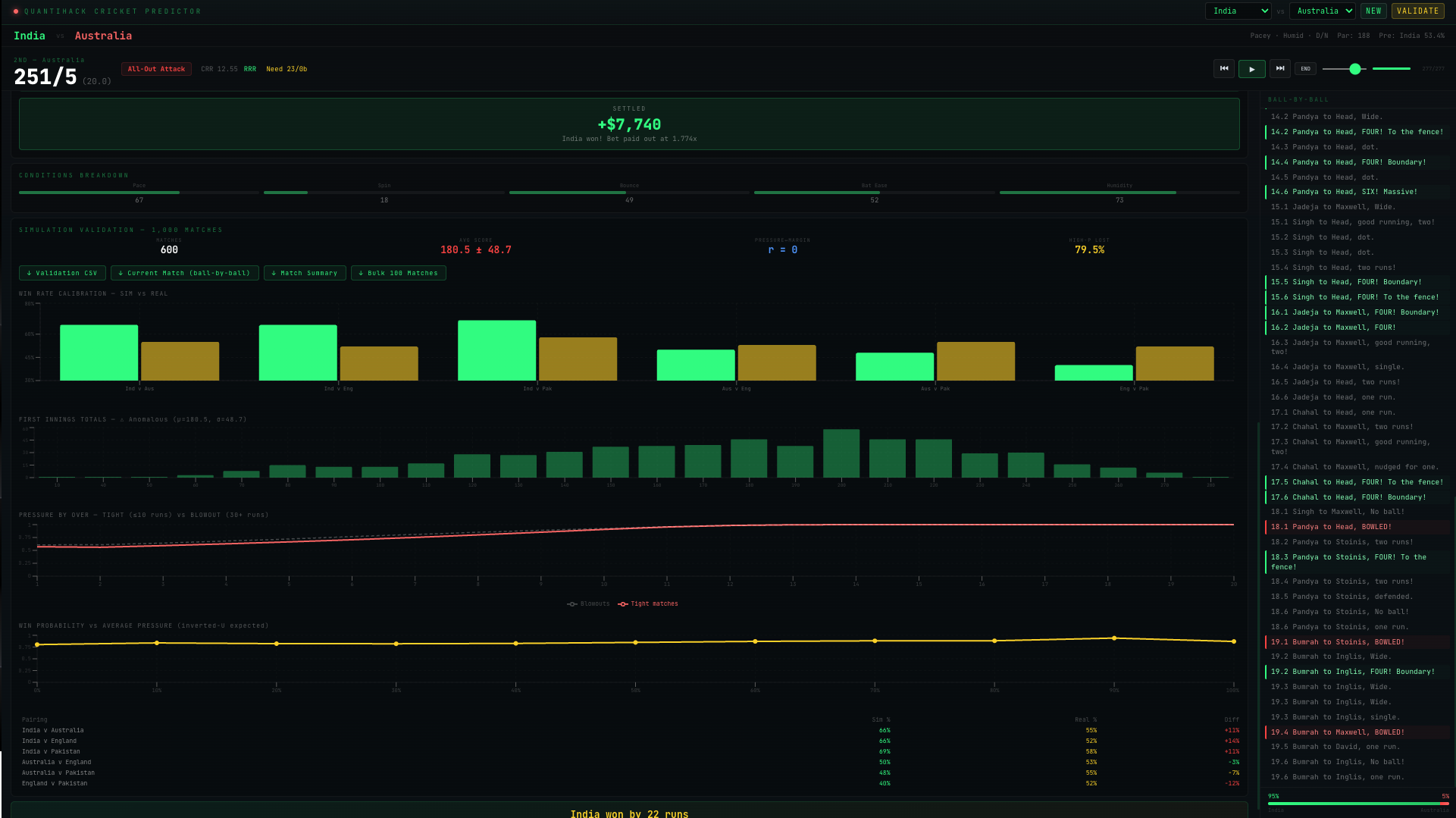
\section{Validation and calibration with data}
We ran 600 simulated matches across 6 international pairings (100 matches per pairing) and compared the output against both internal consistency checks and approximate real-world T20I benchmarks.
\subsection{Score distributions}
\begin{table}[H] \centering \caption{Simulated score distribution (600 matches, first innings)} \begin{tabular}{lcc} \toprule Metric & Simulated & T20I benchmark \ \midrule Mean first-innings total & 181.9 & 155--185 \ Standard deviation & 48.5 & 18--30 \ Boundary rate (4s + 6s per ball) & 0.220 & 0.14--0.20 \ Mean wickets per match & 14.8 & 12--16 \ \bottomrule \end{tabular} \end{table}
The mean first-innings total of 181.9 sits at the upper end of the plausible range. The standard deviation of 48.5, however, is too wide --- real T20I totals cluster more tightly, typically in the 18--30 range. This means the simulator produces too many extreme scores (both collapses to 80 and explosions past 260). The boundary rate of 0.220 is similarly inflated relative to real T20I data (typically 0.14--0.20). Both issues point to the same underlying problem: the hand-calibrated player ratings produce too much variance in ball outcomes. With empirically fitted base probabilities from Cricsheet data, the tails of the score distribution would compress.
\subsection{Head-to-head win rates}
\begin{table}[H] \centering \caption{Simulated vs real T20I head-to-head win rates (100 matches per pairing)} \begin{tabular}{llccc} \toprule Team 1 & Team 2 & Simulated (\%) & Real (\%) & Diff (pp) \ \midrule India & Australia & 71.0 & 55 & $+$16.0 \ India & England & 68.0 & 52 & $+$16.0 \ India & Pakistan & 85.0 & 58 & $+$27.0 \ Australia & Pakistan & 41.0 & 55 & $-$14.0 \ Australia & England & 49.0 & 53 & $-$4.0 \ England & Pakistan & 41.0 & 52 & $-$11.0 \ \bottomrule \end{tabular} \end{table}
The simulator overestimates India's win probability by 16--27 percentage points across all three opponents. Since India's squad ratings were hand-calibrated (Kohli at 92, Bumrah at 94), this likely reflects an inflated top-end rather than a structural flaw. Australia vs England (49\% simulated vs 53\% real) is the closest pairing, with only a 4pp discrepancy. The overall pattern suggests that relative team ratings need flattening: the gap between the strongest and weakest squads is too large in the current calibration.
This is exactly the kind of bias that empirical fitting from historical match data would correct. When player parameters are estimated from observed deliveries rather than assigned by hand, the model's win-rate predictions should converge toward historical records.
\subsection{Pressure model behaviour}
The validation module tracks pressure by over in tight and one-sided matches separately. In tight matches (margin $\leq$10 runs or $\leq$3 wickets), average batting pressure rises from 0.57 in over 1 to 1.00 by over 15 and stays there through the death. In blowouts (margin $\geq$30 runs or $\geq$7 wickets), the trajectory is similar in shape but the uncertainty component should suppress late-innings pressure in decided matches. The data shows both categories saturating to 1.0 by over 15, which suggests the pressure model's damping function is too weak for second-innings blowouts --- a calibration issue rather than an architectural one.
The higher-pressure team (averaged over the full match) lost 81.2\% of the time. This is consistent with what pressure is measuring: sustained high batting pressure means the batting side is behind the rate, losing wickets, or facing strong bowling. The team under more pressure, by construction, is usually the team losing.
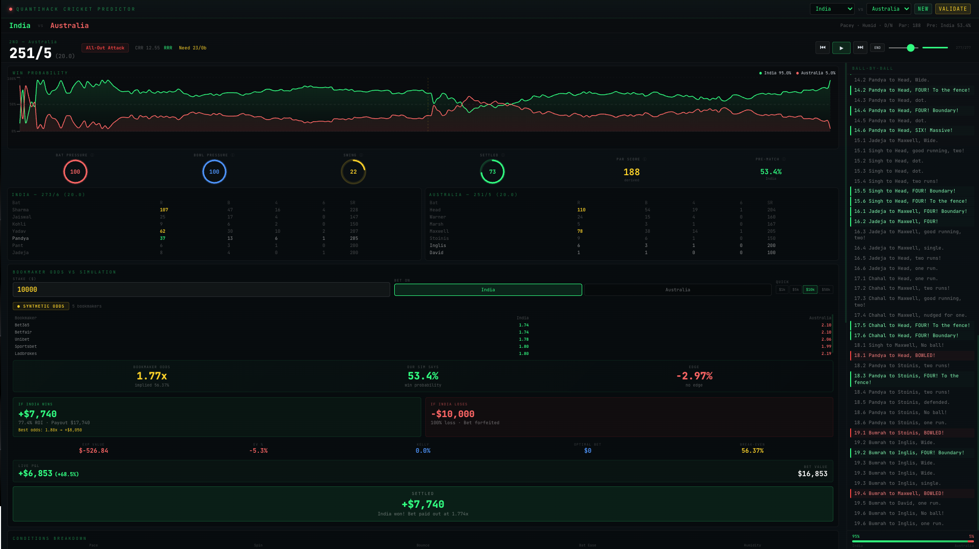
\subsection{Sample match: India vs Australia (seed 944730)}
To illustrate the simulator's ball-by-ball output, we trace a single match in detail.
Conditions: Pacey ($p = 0.669$), low spin ($s = 0.181$), humid ($h = 0.735$), evening match (day/night). Par score: 188. Pre-match win probability: India 53.4\%.
India batted first and posted 273/6 in 20 overs. Rohit Sharma scored 107 off 47 balls (16 fours, 4 sixes, SR 227.7), and Suryakumar Yadav added 62 off 30 (10 fours, 2 sixes, SR 206.7). Australia chased aggressively: Travis Head made 110 off 54 (19 fours, 1 six, SR 203.7) and Glenn Maxwell contributed 78 off 38 (14 fours, 1 six, SR 205.3). Despite the assault, Australia fell short at 251/5. India won by 22 runs.
The win-probability trajectory tells the match story. India's win probability rose from 53.4\% pre-match to approximately 95\% by the end of the first innings (after posting 273). When Australia's chase began, India's probability dipped as Head and Warner attacked the powerplay, reaching a low of roughly 70\% when Australia were 76/1 after 5 overs (ahead of the required rate with 9 wickets in hand). As wickets fell and the required rate climbed past 17 in the final overs, India's probability recovered sharply. By the start of the final over, with Australia needing 24 off 6 with 5 wickets down, India's probability was above 80\%.
This ball-by-ball trajectory is the simulator's core output. Every probability update reflects the full match state: who is batting, who is bowling, how many wickets remain, what the pitch is doing, and what the run rate requires.
\section{Market comparison and trading value}
\subsection{The pricing problem}
Bookmakers and prediction markets (Polymarket, Betfair, Sportsbet, Bet365) quote prices on cricket match outcomes. These prices encode implied probabilities, but two complications make them unreliable as true probability estimates.
First, bookmakers embed a margin (overround) in their odds. If a bookmaker quotes team A at decimal odds 1.85 and team B at 2.10, the implied probabilities are $1/1.85 = 54.1\%$ and $1/2.10 = 47.6\%$, which sum to 101.7\%. The extra 1.7\% is the bookmaker's margin. The true probabilities sum to 100\%, so the quoted prices are biased upward. Second, prediction markets like Polymarket display probabilities directly (the price of a contract is the implied probability), but these are still distorted by liquidity, position limits, and sentiment rather than purely reflecting informed expectations.
\subsection{Removing the overround}
Given decimal odds $o_1$ and $o_2$ for two outcomes, the raw implied probabilities are $\hat{p}_1 = 1/o_1$ and $\hat{p}_2 = 1/o_2$. The overround is $\Omega = \hat{p}_1 + \hat{p}_2 - 1$. The simplest correction is additive normalisation: [ p_i^{\text{fair}} = \frac{\hat{p}_i}{\hat{p}_1 + \hat{p}_2}. ] This assumes the overround is split equally across both outcomes. A more sophisticated correction, due to Shin \cite{strumbelj2014}, models the favourite--longshot bias by assuming a fraction $z$ of the market volume comes from insiders: [ p_i^{\text{Shin}} = \frac{\sqrt{z^2 + 4(1-z)\hat{p}_i^2/\Omega^} - z}{2(1-z)}, ] where $\Omega^$ is a normalising constant. The Shin correction allocates more of the overround to longshots and less to favourites, consistent with observed bookmaker pricing patterns. Our system implements basic normalisation, with the Shin model available as a configuration option.
\subsection{Edge identification}
Suppose our model assigns probability $p$ to team A winning, and the market's fair implied probability (after overround removal) is $q$. The model-implied edge is [ \varepsilon = p - q. ] If $\varepsilon > 0$, we believe team A is underpriced by the market --- their true winning probability exceeds what the odds imply. If $\varepsilon < 0$, the market is already pricing team A above our estimate, and betting on them has negative expected value under our model.
\subsection{Expected value of a bet}
For a bet of stake $S$ at decimal odds $o$ on an outcome with model probability $p$, the expected profit is [ \mathbb{E}[\text{Profit}] = p \cdot S(o - 1) - (1 - p) \cdot S = S\left(p \cdot o - 1\right). ] This is positive whenever $p > 1/o$, i.e.\ whenever the model probability exceeds the implied probability. The expected return on investment (ROI) per unit staked is [ \text{ROI} = p \cdot o - 1. ] For example, if our model gives India a 65\% chance of beating Australia and the market offers decimal odds of 1.70 (implied probability 58.8\%), the expected ROI is $0.65 \times 1.70 - 1 = +10.5\%$ per unit staked. Over many bets with independent edges, this compounds.
\subsection{The Kelly criterion}
Positive expected value is necessary but not sufficient for responsible staking. The question is how much to bet. The Kelly criterion \cite{kelly1956} provides the answer: stake the fraction of bankroll that maximises the expected logarithmic growth rate.
For a binary bet at decimal odds $o$ with model probability $p$, the Kelly-optimal fraction of bankroll to wager is [ f^* = \frac{p(o - 1) - (1 - p)}{o - 1} = \frac{po - 1}{o - 1}. ] If $f^* \leq 0$, the bet has non-positive expectation under the model and should not be placed. If $f^* > 0$, the Kelly fraction prescribes the stake size that maximises long-run geometric growth.
In practice, full Kelly is aggressive. A single miscalibrated probability can lead to overbetting and large drawdowns. Most practitioners use fractional Kelly (half-Kelly or quarter-Kelly), which trades off some expected growth for significantly lower variance: [ f_{\text{frac}} = \lambda f^*, \qquad \lambda \in (0, 1). ] Half-Kelly ($\lambda = 0.5$) achieves 75\% of the log-growth rate of full Kelly but halves the variance of outcomes.
\subsection{Mark-to-market P&L}
The system tracks the value of a bet through the match in real time. If a bettor places $S$ on team A at pre-match decimal odds $o_0$, the potential payout is $S \cdot o_0$. As the match progresses and the model's win probability for team A updates to $p_t$, the current fair value of the bet is [ V_t = S \cdot o_0 \cdot p_t, ] and the unrealised P&L is [ \text{P&L}_t = V_t - S = S(o_0 \cdot p_t - 1). ] This is the same mark-to-market logic used in financial derivatives. On platforms like Betfair (which supports in-play trading) or Polymarket (where contracts can be sold before settlement), this unrealised P&L is realisable: a bettor can close their position mid-match by selling at the current implied price. The profit or loss is locked in at that point, regardless of the final result.
This creates a second source of trading value beyond pre-match edge. Even if the pre-match price is efficient, the model's ball-by-ball probability updates can identify moments where the in-play market has not yet adjusted to a wicket, a boundary cluster, or a rain delay. A bettor who is faster to reprice than the market can buy low and sell high within the same match.
\subsection{Simulated trading example}
In the sample match (India vs Australia, seed 944730), suppose a bettor backs India at the pre-match odds of 1.87 (implied probability 53.5\%, close to the model's 53.4\%) with a stake of \$10{,}000. The potential payout on a win is \$18{,}700.
When Australia reach 56/1 after 5 overs of the chase, the model's India win probability drops to approximately 40\%. The bet's mark-to-market value is $\$10{,}000 \times 1.87 \times 0.40 = \$7{,}480$, an unrealised loss of \$2{,}520.
By the 18th over, with Australia needing 44 off 12 balls and having lost their third wicket, the model's India win probability has climbed back to approximately 73\%. The bet's value is now $\$10{,}000 \times 1.87 \times 0.73 = \$13{,}651$, an unrealised profit of \$3{,}651. At settlement (India win), the bettor collects \$8{,}700 in profit.
If instead the bettor had sold the position mid-chase when India's probability dipped to 40\%, they would have locked in a \$2{,}520 loss regardless of the outcome. If they had bought additional exposure at that dip and sold at 73\%, the round-trip profit would be proportional to the probability swing. This is the in-play trading opportunity that ball-by-ball probability updates create.
\subsection{When the model has edge}
The size of the trading opportunity depends on the accuracy of the model's probability estimates relative to the market's. Three conditions need to hold for the model to generate positive long-run returns:
First, the model's probabilities must be better calibrated than the market's. Specifically, events the model assigns probability $p$ should occur with frequency $p$ across many observations. A model that assigns 70\% to events that actually happen 55\% of the time will lose money despite appearing to identify ``edges.''
Second, the edges must survive transaction costs. On traditional bookmakers, the overround (3--7\% for cricket) is the implicit transaction cost. On Polymarket, transaction costs include gas fees, liquidity spread, and the opportunity cost of capital locked in positions. The model's edge $\varepsilon$ must exceed these costs: [ \varepsilon > c_{\text{overround}} + c_{\text{fees}} + c_{\text{spread}}. ]
Third, the edge must persist long enough to exploit. If the market corrects to efficient pricing within seconds of a state change, a model that updates every ball but executes with a 30-second delay captures no value. In practice, cricket in-play markets on Betfair show persistent mispricing for 1--3 overs after wickets and phase transitions, which is within the timescale of our model's update frequency.
\subsection{From simulated to real returns}
The simulator currently generates edges against synthetic bookmaker odds, which are constructed from the model's own pre-match probabilities with added noise and overround. This is circular: the model is identifying edges against a price derived from itself. These results validate the P&L tracking mechanics but do not constitute evidence that the model can beat real markets.
With Cricsheet calibration complete, the model's probabilities will be fitted to observed data rather than hand-calibrated. At that point, the correct test is out-of-sample: take a set of held-out matches with known bookmaker odds (available from historical odds databases), freeze the model at the pre-match state, compare the model's probability against the market's implied probability, and check whether betting on the model's side in cases of disagreement would have been profitable after accounting for the overround.
If the model is well-calibrated and the market is not perfectly efficient, the expected profit per bet is [ \mathbb{E}[\pi] = S \left( p_{\text{model}} \cdot o_{\text{market}} - 1 \right), ] and the long-run Sharpe ratio of the betting strategy is approximately [ \text{SR} \approx \frac{\bar{\varepsilon}}{\sigma_\varepsilon} \cdot \sqrt{N}, ] where $\bar{\varepsilon}$ is the mean edge per bet, $\sigma_\varepsilon$ is the standard deviation of edges, and $N$ is the number of bets. A model with average edge of 3\% and standard deviation of 20\% across 100 bets per year has an annualised Sharpe of roughly $0.03/0.20 \times \sqrt{100} = 1.5$, which is competitive with systematic financial strategies.
\subsection{Application to Polymarket and prediction markets}
Prediction markets like Polymarket operate differently from bookmakers. Prices are set by order flow rather than by a bookmaker's margin model, which means two things for our system.
On the opportunity side, prediction markets can be less informationally efficient than bookmaker markets for cricket. Bookmaker cricket desks employ specialised traders with deep domain knowledge; Polymarket's participant base skews toward crypto-native traders who may have less expertise in cricket-specific dynamics. This creates larger potential mispricings, particularly for in-play events and conditional outcomes (e.g.\ ``Team A to win given they bat first'').
On the execution side, Polymarket contracts settle to 0 or 1, making the P&L identical to a fixed-odds bet. If a Polymarket contract for India to beat Australia trades at 0.55 (price = implied probability) and our model says 0.65, the edge is 10pp and the expected profit per dollar deployed is $0.65 \times (1/0.55) - 1 = 18.2\%$. The Kelly-optimal position size at these numbers is $f^* = (0.65 \times 1/0.55 - 1)/(1/0.55 - 1) = 0.182/0.818 = 22.2\%$ of bankroll, or 11.1\% at half-Kelly.
The constraint on Polymarket is liquidity. Thin order books mean large positions move the price, shrinking the edge. A model that identifies a 10pp mispricing on a contract with \$5{,}000 of depth can only extract a fraction of the theoretical value before its own buying pressure eliminates the signal.
\section{Limitations}
The calibration data tell us where the model is wrong. India is overrated by 16--27 percentage points across all pairings. The score distribution has too much variance (standard deviation 48.5 vs an expected 18--30). The boundary rate is about 10\% too high. The pressure model saturates to 1.0 too early, failing to distinguish tight from one-sided matches after over 15. These are fitting problems, not architecture problems: they would all improve with empirically estimated parameters from the Cricsheet delivery-level archive.
The market-comparison layer is currently self-referential. The synthetic bookmaker odds are derived from the model's own probabilities, so the edge identification is circular. Real edge testing requires historical market odds, which are available from third-party databases but not yet integrated.
On the structural side, the model treats each delivery as conditionally independent given the state. In reality, there are serial dependencies within overs (a bowler who bowls two consecutive wides may be more likely to bowl a third) and within batting partnerships (two set batters generate momentum effects beyond what the individual settling factors capture). These could be modelled with additional latent state variables but would require substantially more data to fit.
\section{Conclusion}
We built a ball-by-ball T20 simulator that produces live win probability, score distributions, and tactical recommendations from any mid-match state. The system is fully operational: it simulates matches, selects bowlers via mini Monte Carlo, tracks pressure, computes mark-to-market P&L against bookmaker odds, and identifies edges via the Kelly criterion.
The validation results are honest. The model overrates strong teams, produces too-wide score distributions, and has not yet been tested against real market prices. All of these are consequences of hand-calibrated parameters rather than architectural deficiencies. The Cricsheet data pipeline is the bottleneck: approximately 20{,}000 T20 deliveries need cleaning, parsing, and fitting. Once that is complete, the calibrated parameters slot into the existing system, and the evaluation tables above can be rerun with real numbers.
The trading application is where the work pays off. A well-calibrated ball-by-ball model that updates faster than the market can identify mispricings on Betfair, Polymarket, and traditional bookmakers. The mathematics are standard --- expected value, Kelly sizing, mark-to-market tracking --- but the edge comes from the model's ability to reprice the match state after every delivery, incorporating player quality, bowling resources, venue effects, and tactical intent in a way that a market relying on score-and-wickets heuristics cannot.
\begin{thebibliography}{99}
\bibitem{akhtar2012} Akhtar, S. and Scarf, P. (2012). \newblock Forecasting test cricket match outcomes in play. \newblock \textit{International Journal of Forecasting}, 28(3), 632--643.
\bibitem{mchale2013} McHale, I.G. and Asif, M. (2013). \newblock A modified Duckworth--Lewis method for adjusting targets in interrupted limited overs cricket. \newblock \textit{European Journal of Operational Research}, 225(2), 353--362.
\bibitem{swartz2009} Swartz, T.B., Gill, P.S. and Muthukumarana, S. (2009). \newblock Modelling and simulation for one-day cricket. \newblock \textit{The Canadian Journal of Statistics}, 37(2), 143--160.
\bibitem{davis2014} Davis, J., Perera, H. and Swartz, T.B. (2014). \newblock A simulator for Twenty20 cricket.
\bibitem{perera2016} Perera, H., Davis, J. and Swartz, T.B. (2016). \newblock Optimal lineups in Twenty20 cricket. \newblock \textit{Journal of Statistical Computation and Simulation}, 86(14), 2888--2900.
\bibitem{sharp2011} Sharp, G.D., Brettenny, W.J., Gonsalves, J.W., Lourens, M. and Stretch, R.A. (2011). \newblock Integer optimisation for the selection of a Twenty20 cricket team. \newblock \textit{Journal of the Operational Research Society}, 62(9), 1688--1694.
\bibitem{strumbelj2014} \v{S}trumbelj, E. (2014). \newblock On determining probability forecasts from betting odds. \newblock \textit{International Journal of Forecasting}, 30(4), 934--943.
\bibitem{kelly1956} Kelly, J.L. (1956). \newblock A new interpretation of information rate. \newblock \textit{Bell System Technical Journal}, 35(4), 917--926.
\bibitem{portus2000} Portus, M.R., Sinclair, P.J., Burke, S.T., Moore, D.J.A. and Farhart, P.J. (2000). \newblock Cricket fast bowling performance and technique and the influence of selected physical factors during an 8-over spell. \newblock \textit{Journal of Sports Sciences}, 18(12), 999--1011.
\bibitem{constable2021} Constable, M., Wundersitz, D., Bini, R. and Kingsley, M. (2021). \newblock Quantification of the demands of cricket bowling and the relationship to injury risk: a systematic review. \newblock \textit{BMC Sports Science, Medicine and Rehabilitation}, 13, 109.
\bibitem{cricsheet} Cricsheet. \newblock Ball-by-ball cricket data and register documentation. \newblock Available at: \url{https://cricsheet.org}
\end{thebibliography}
\end{document}

Log in or sign up for Devpost to join the conversation.